
Tom Goddard
Oct 14, 2013
Review of some molecular surface calculation methods to see what is best to use in Chimera 2 as a replacement for MSMS. MSMS crashes on most structures larger than 10,000 atoms. Will look at distance grid SES surfaces, Gaussian surfaces, level set molecular surface algorithm (LSMS), PyMol surface code, maybe hard-spheres with boundary smoothing (as done in Chimera masking code).
I cooked up a distance grid solvent excluded surface calculation in Chimera using just 100 lines of Python and 50 lines of C++ and got smooth looking surfaces, with the same compute time as MSMS and working on molecules of any size. This looks like the best candiate to replace MSMS.
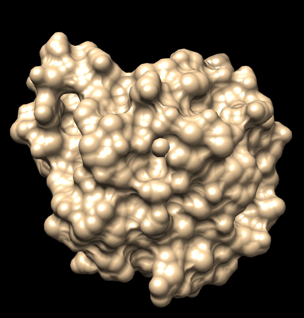
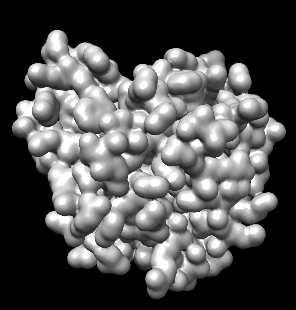
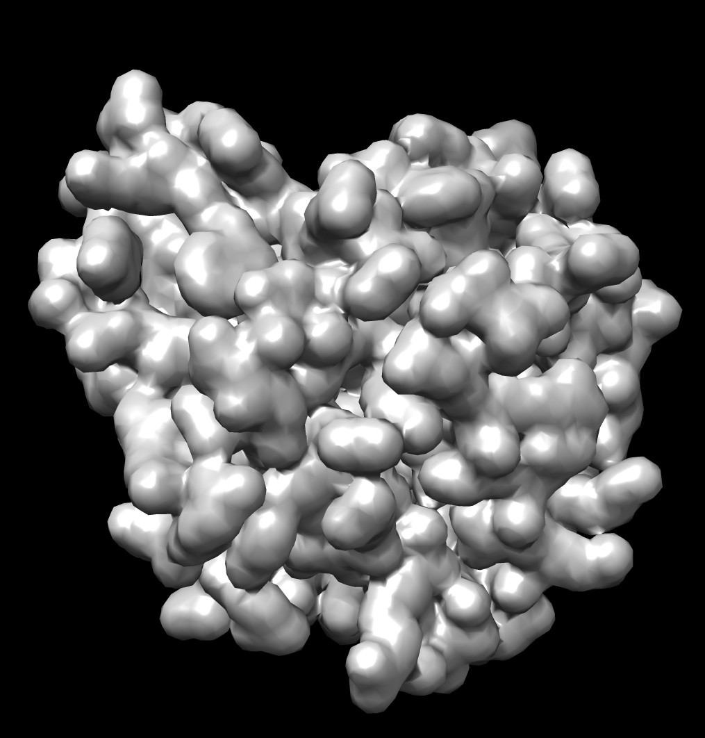
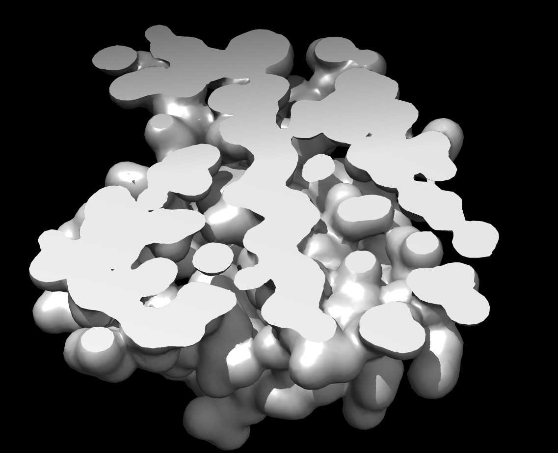
Shape comparison of MSMS and distance grid surfaces|
|
|
|
| MSMS, vertex density 2, 1a0m | Distance grid, 0.5A spacing, 1a0m | Distance grid, 0.2A spacing, 1a0m |
The distance grid surfaces as grid spacing approaches zero produce the exact solvent excluded surface. At grid spacing 0.5 Angstroms they appear smoother than MSMS surfaces, requiring about the same computation time as MSMS. At grid spacing 0.2 Angstroms they show more fine detail, but still not as much as the analytic MSMS surface calculation. I think for the common uses of molecular surfaces the smoother 0.5 Angstrom distance grid surface may serve better than MSMS by avoiding distracting superfluous high detail in the webbed appearance.
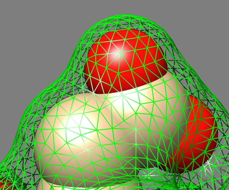
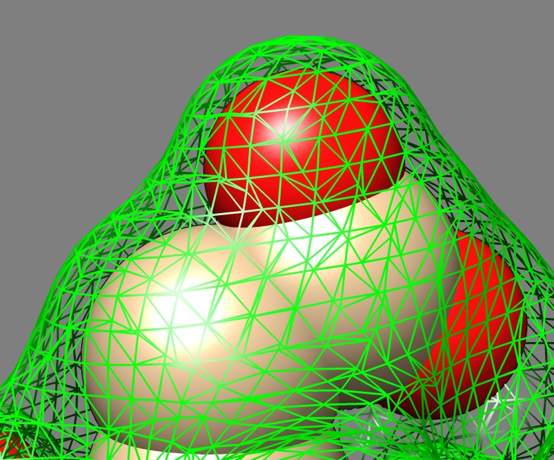
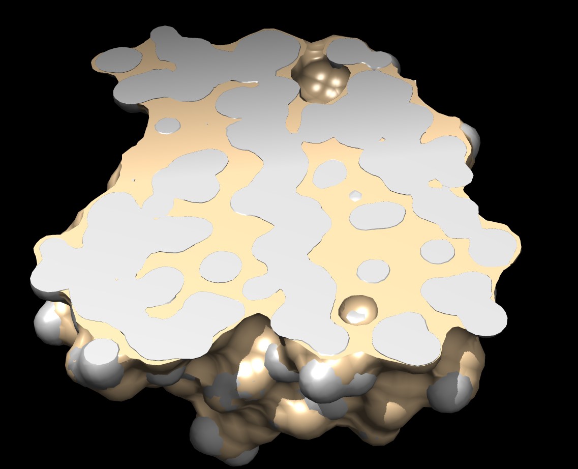
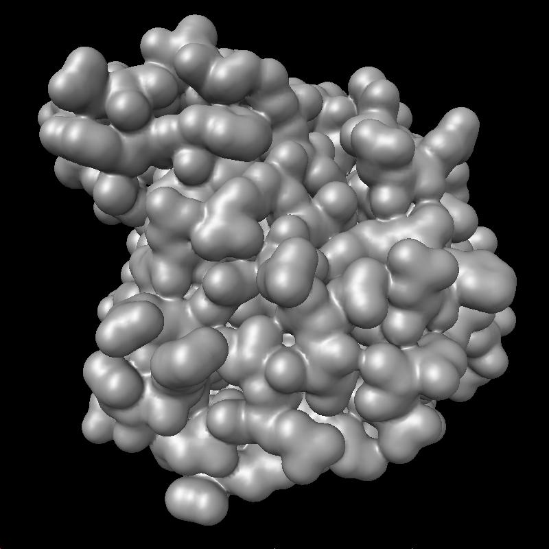
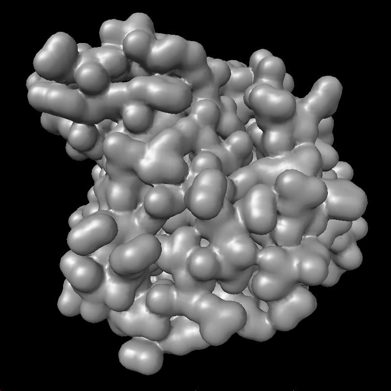
Shape comparison to MSMS vertex density 20 surface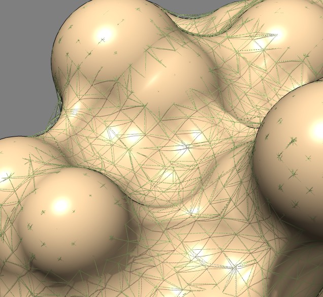
| 
| 
|
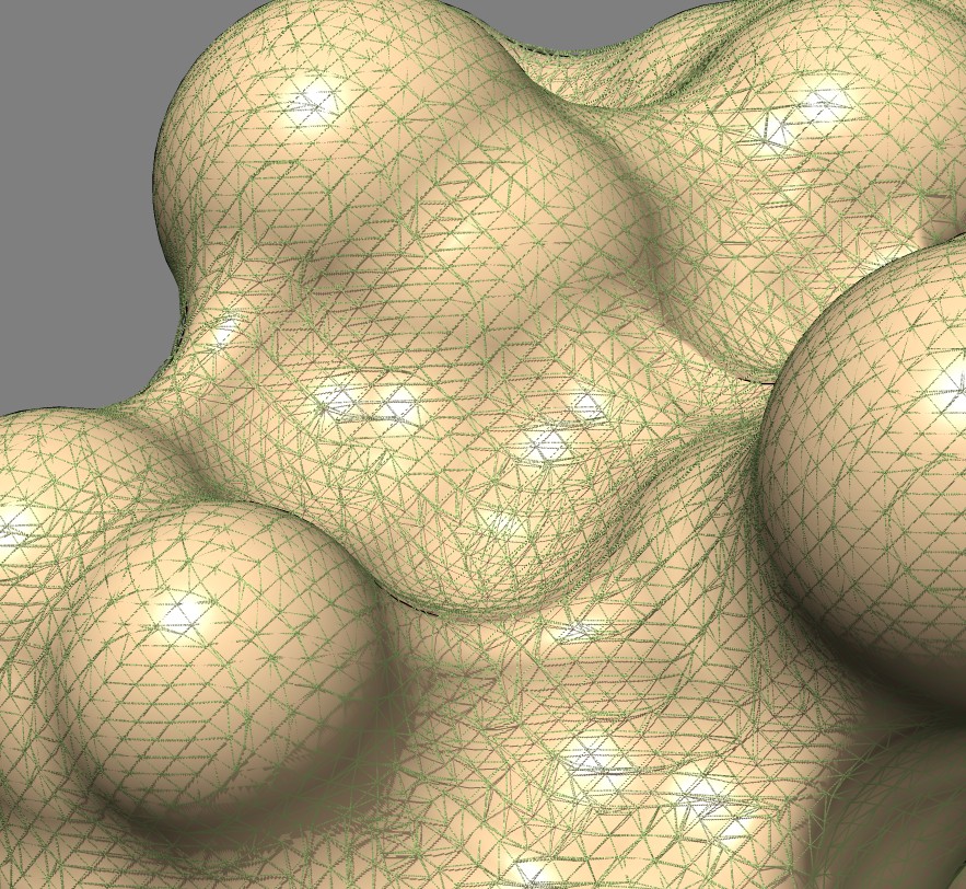
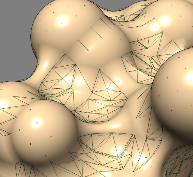
| 0.5A distance grid mesh (green), MSMS vertex density 20 surface (tan) | 0.2A distance grid mesh | MSMS vertex density 2 mesh |
The distance grid meshes are very close to the MSMS surface. Differences in shape between the 0.5 Angstrom distance grid surface and a high vertex density MSMS surface are comparable to the differences between a normal vertex density MSMS surface (dens = 2) and high density MSMS surface (dens = 20).
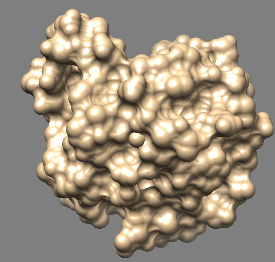
Distance grid 0.5A, ribosome, 100,000 atoms (1jj2), ~30 seconds. MSMS calculation fails.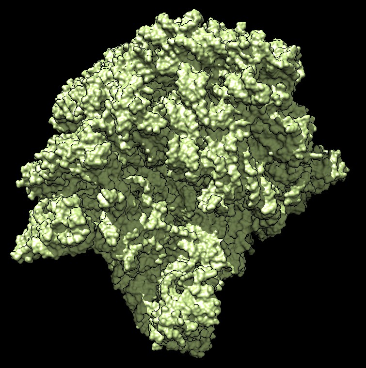
There are no numerical instabilities with the distance grid calculation so surfaces can be computed for arbitrarily large molecular structures. The memory use allows handling very large molecules, using a single 3-d grid of 32-bit floating point values bounding the molecule at the specified grid spacing. For a 0.5 Angstrom grid the 100,000 atom ribosome structure 1jj2 used a grid size of 463 by 463 by 371 (80 million grid points), taking 320 Mbytes of memory, and 30 seconds to compute with unoptimized code.
The distance grid surfaces at 0.5 Angstrom grid spacing have about 3 times more triangles than an MSMS surface with vertex density 2. (3fx2, MSMS 22546 triangles, distance grid 66828 triangles). This is not surprising since the MSMS triangulation is carefully tailored to the geometry of the spherical and toroidal patches, while the marching cubes triangulation of the distance grids is irregular with many skinny triangles. The 0.5 Angstrom distance grid surface of ribosome 1jj2 (~100,000 atoms) contains 5.3 million triangles. Rendering with current graphics cards can handle about 20 million triangles before slowing down. Surfaces in Chimera take 24 bytes per triangle, so 5 million triangles will consume 100 Mbytes.
Chimera associates a patch of surface with each atom. A drawback of the distance grid surfaces is that the atom patch may have jagged sawtooth edges. The surface triangulation for distance grid surfaces comes from the marching cubes algorithm. MSMS does a uniform triangulation of the toroidal patches that separate atoms that creates a smooth dividing line between atom patches.
| 
| 
|
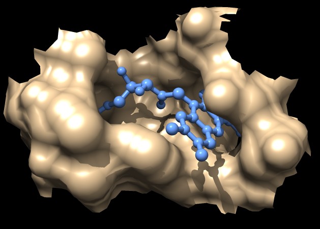
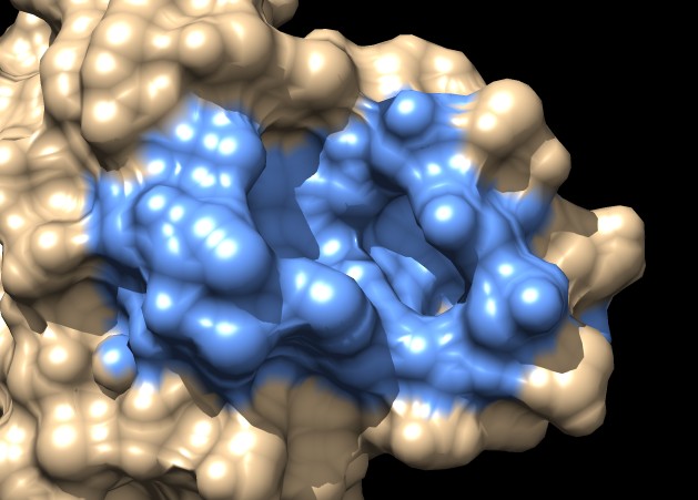
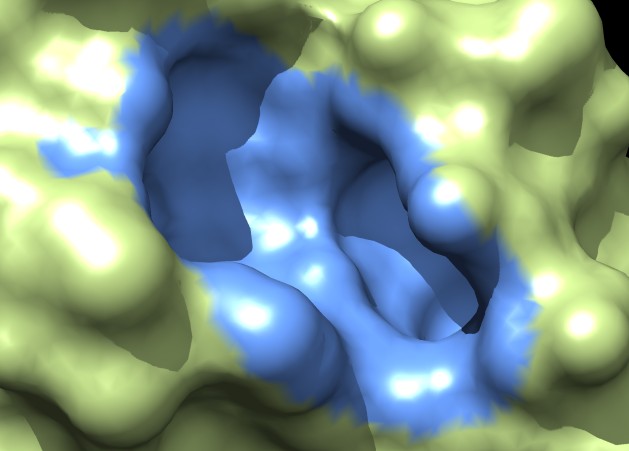
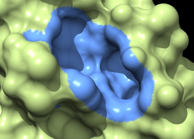
| MSMS surface for residues within 4A of ligand, 3fx2 | Distance grid surface within 4A of ligand, 3fx2 | Distance grid surface within 4A of ligand, 0.2A grid spacing |
The example images show that both MSMS and distance grid surface patches have jagged perimeters. A smaller grid spacing can produce smaller sawteeth. Probably we need to allow patch display that slices surface triangles in half to allow smooth edges, as is done by the "measure contactArea" command.
| 
| 
|
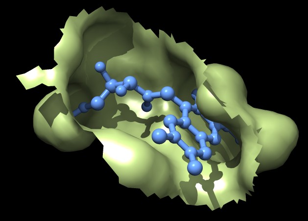
| MSMS surface for residues within 4A of ligand, 3fx2 | Distance grid surface within 4A of ligand, 3fx2 | Distance grid surface within 4A of ligand, 0.2A grid spacing |
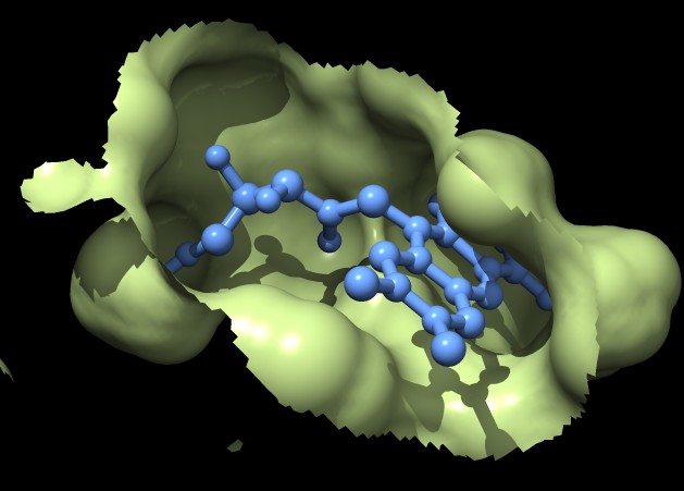
Coloring a ligand pocket shows similar jagged perimeter. The example images colored MSMS surface patches for residues within 4 Angstroms of the ligand for 3fx2, and colored the distance grid surface triangles within 4 Angstroms of the ligand. A smaller grid spacing produces smaller sawteeth. Again a cleaner smooth perimeter would require triangle splitting for both surfaces. Duplicating vertices at the boundary lines and using triangle splitting would allow sharp and smooth edges.
| 
|
| MSMS mesh, vertex density 10, atoms at 75% radius | Distance grid mesh, spacing 0.3 A |
The MSMS mesh is aligned with the atoms so it could give smoother boundaries for atom patches. If surface vertices lie exactly at a boundary between atoms, such vertices are associated with just one atom in an asymmetric way. Also color is linearly interpolated between vertices so a sharp color transition is not possible in Chimera.
Here's a description of the grid SES algorithm. First a simple approach. Take each atom sphere, expand it by the probe radius, and mark grid points inside those spheres with ones, outside will be 0. The boundary between ones and zeros is the solvent accessible surface (SAS), that is where the center of the probe sphere rolling over the atoms can reach. The solvent excluded surface is the boundary of where the surface of the rolling probe sphere can reach. To get that we can place a probe sphere at every grid point on the boundary of the solvent accessible grid -- in other words at every grid point with value 0 that is adjacent to a grid point with value 1. Set the grids points inside all such probe spheres to zero. Now the grid boundary between ones and zeros is the solvent excluded surface. Using marching cubes we can compute that surface (say at a contour level of 0.5). That surface will look horrible with large stair-step artifacts. That is what happens when you try to surface a zero/one mask.
The insight I had yesterday was to make two improvements that make the result much smoother. Instead of a grid of 0 and 1 values, use floating point values that measure the distance from the surface with positive values being outside, negative values being inside, and zero right on the surface. Now the first step is to put the atom spheres expanded by the probe radius on the grid and set grid point values to the distance from that sphere surface within a grid subregion that is a little bigger than the sphere. When I add multiple spheres set grid values as the minimum of the sphere surface distance and the current grid value. Now I compute a contour surface of this distance grid at threshold level 0 and it produces a very smooth solvent accessible surface. For the second step of placing a probe sphere at each boundary point, instead of centering them on grid points, center them on each vertex of the calculated contour solvent accessible surface. This much more accurately centers them on the boundary. Erase the original grid and compute a new distance to surface grid using all the probe spheres centered at the solvent accessible surface vertices. Compute a contour surface of this new distance grid to get the smooth solvent excluded surface. It actually gives the solvent excluded surface and another surface a probe diameter further away. I eliminate the extra surface(s) by checking how close one vertex or each connected surface component is to the original atom spheres. If the vertex is 2 probe radii or more away (I use 1.5*probe radius) then it is an extra surface component and I delete it. There may be large internal pockets and they can have extra surface components, so I test one vertex of each connected surface component to eliminate the non-SES pieces. That's it.
Using the distance from surface maps for a set of spheres two times produces a remarkably smooth result. Although I said it is 150 lines of code (100 in Python, 50 in C++) that doesn't count the existing code in Chimera I called, like marching cubes contour surface calculation, and connected surface component calculation. But it was just 150 new lines of code.
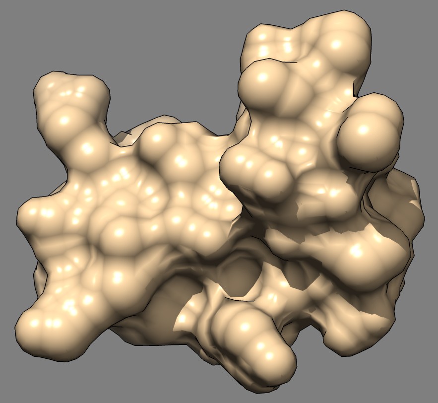
Solvent excluded surfaces are obtained by rolling a probe sphere (usual radius 1.4 Angstroms) over a molecule and taking the boundary of the reachable volume of the probe. The MSMS code used by Chimera computes this type of surface.
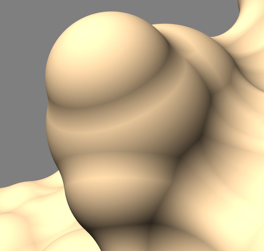
Solvent excluded surfaces have a webbed appearance. This appearance comes from the "toroidal" patches. These occur when the probe sphere rolls in while touching two nearby atoms sweeping out a donut also called a torus. This creates a concave patch that fills the gap between the two atoms. If the two atoms are far apart the concave segment looks like a ligament. These are seen all over the surface and give it the intricate "webbed" appearance.
Between two close atoms the toroidal surface looks like a band. An odd feature is that this band does not blend smoothly with the atom spheres. The fact that these bands, and all of the toroid segments show a sharp dividing line with the spheres that they smoothly join to adds to the complex appearance of the surface. The dividing lines are obvious variations in shading while the sphere and toroid surfaces join with matching tangent planes. I thought these sharp visual dividing lines were a bug in the surface normals and spent a few hours to figure out that it is actually the correct appearance. The sharp divisions seem to add undesirable complexity and a visually smooth join with no sharp demarcation between convex and concave regions might make a more pleasing surface.
| 
|
| 3fx2, MSMS, vertex density 100 | Toroidal band, diffuse lighting, no specular |
Here's an explanation of the clear visual line between toroid and sphere patches. If you move along the surface from a sphere to a toroid in a straight line perpendicular to the boundary between the sphere and toroid, the surface normal vector rotates at a constant rate while on the sphere and then switches to rotating at a different constant rate when you cross to the toroidal patch. The constant rates of the rotation on the sphere and toroid have opposite signs. A graph of the angle the normal makes to a normal vector at the crossing point would be a saw tooth with a linearly rising segment, then a cusp, then a linearly falling segment. The diffuse lighting of the surface is computed as a dot product of this normal with the light direction and will also be a saw tooth. The result is you will see the light linearly darkening across the surface, then suddenly start to linearly increase when the sphere/toroid boundary is crossed. This will look like a color brightness gradient adjacent to the same gradient in the opposite direction and gives the impression of a distinct line where the reversal in intensity occurs. A general conclusion from this analysis is that a C1 surface (continuous derivatives or tangent planes) gives rise to only C0 color variation (continuous, but derivative of color change across surface can have cusps). So to get smooth lighting variation one needs a C2 surface (second derivatives continuous). Solvent excluded surfaces jump from curvature 1/(atom radius) to curvature -1/(probe radius) discontinuously when crossing from a sphere to a toroid.
Can create a contour surface from a density map obtained by summing Gaussians centered on each atom position. The Chimera "molmap" command does this. It uses the same Gaussian standard deviation (i.e. radius) for all atoms and scales each Gaussian by the element number of the atom.
| 
| 
|
| 3fx2, MSMS, vertex density 2 22546 triangles, 5792 A**2, 0.26 A**2/triangle | 3fx2, molmap, res 3, grid 0.5 139824 triangles, 11740 A**2, 0.08 A**2/triangle | 3fx2, molmap, res 3, grid 0.8 53016 triangles, 11730 A**2, 0.22 A**/triangle |
| 
| 
|
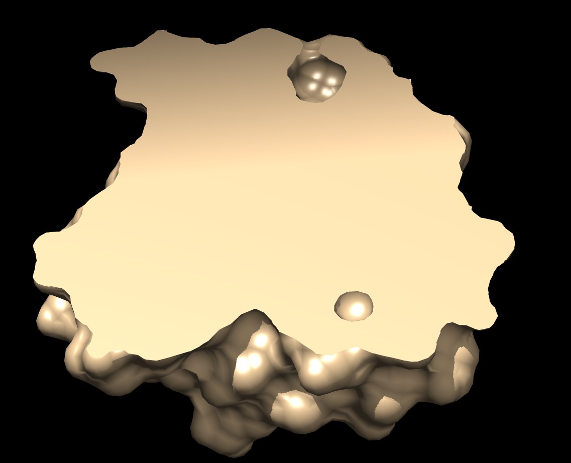
| 3fx2, MSMS, cut | 3fx2, molmap, res 3, grid 0.5, cut | MSMS and molmap cut |
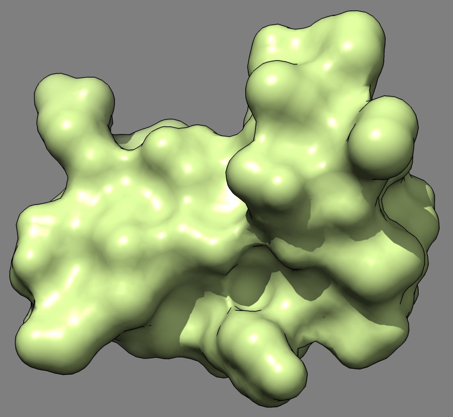
The Gaussian surface described above summed a Gaussian for each atom with each Gaussian having the same standard deviation, and the height scale by the element number. This choice of atom density function was used because it is what the Chimera molmap command does for simulating low resolution electron microscopy maps from atomic models. Other choices might give nicer appearance. For instance, we can vary the Gaussian radius proportional to atom radius and leave all the Gaussian heights equal. Or to control both the radius and the roll-off we can have the atom density be flat out to a radius R then fall-off with a half-Gaussian of specified line width. I tried this last idea. Here is an image.
| 
| 
|
| 3fx2, balls, fall-off sdev=1/(pi*sqrt(2))=0.23, grid 0.3, constant over atom radius - sdev, contour level 0.5. | Ball surface mesh and atoms | Gaussian surface, sdev=3/(pi*sqrt(2))=0.68, grid 0.5, contour level 0.1. |
The balls and Gaussian surfaces are nearly indistinguishable. I had to use finer grid spacing 0.3 A versus 0.5 A on the balls density map to get similarly smooth appearance, probably because the atom density function falls off faster. Both surfaces very closesly approximate the atom spheres.
LSMS (level set molecular surface) computes a solvent excluded molecular surface using a 3-d grid method. It is described in
Efficient molecular surface generation using level-set methods
T. Can, C.I. Chen, Y.F. Wang
J Mol Graph Model. 2006 Dec;25(4):442-54. Epub 2006 Apr 18.
Summary of test results:
| 
|
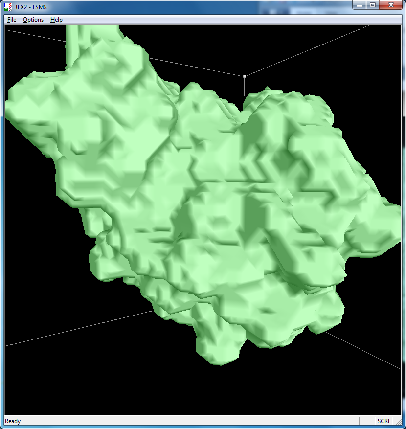
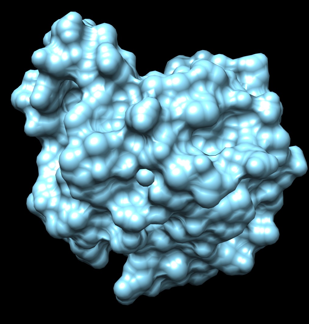
| 3fx2 LSMS, quality 1.7, grid size 64 | 3fx2 Chimera MSMS |
|
| 
| 
|
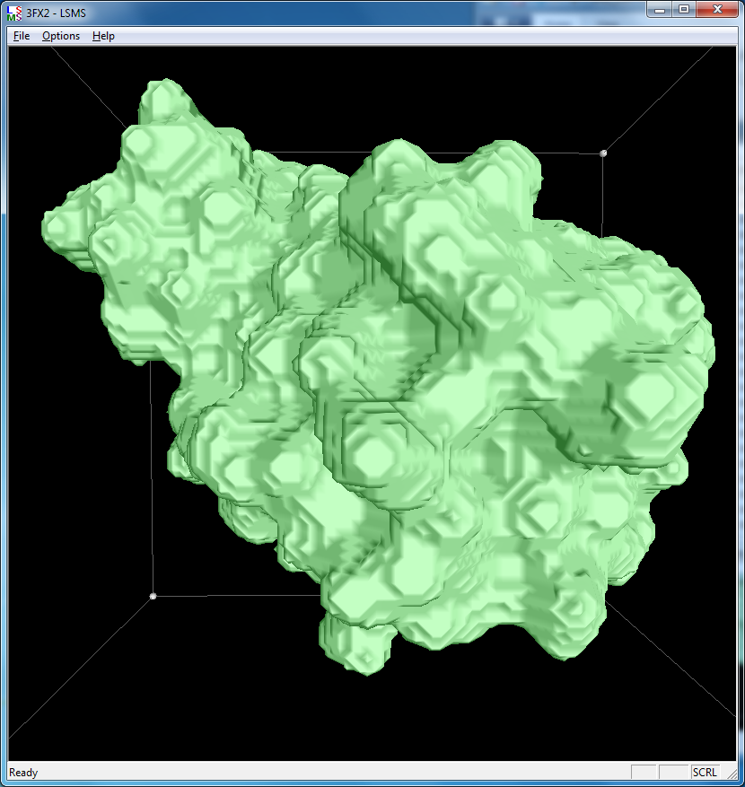
| 3fx2 LSMS, grid size 64, (quality 1.7) | 3fx2 LSMS, grid size 128, (quality 3.4) | 3fx2 LSMS, grid size 256, (quality 6.8) |
| 
| 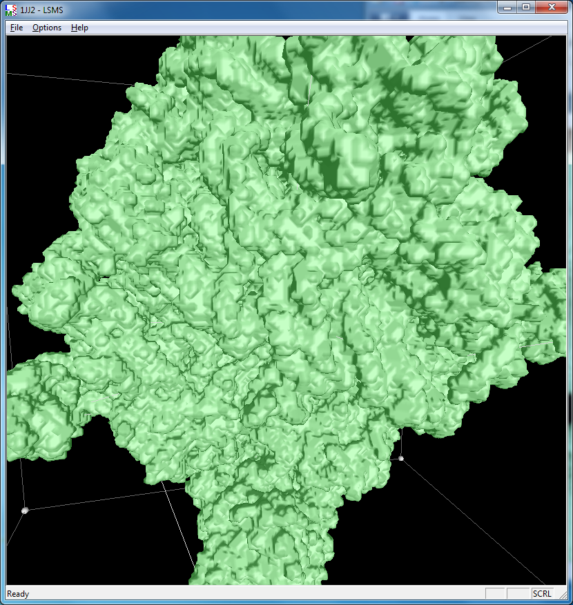
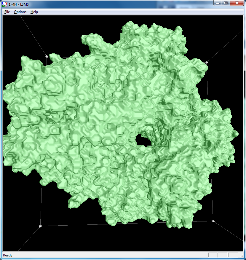
|
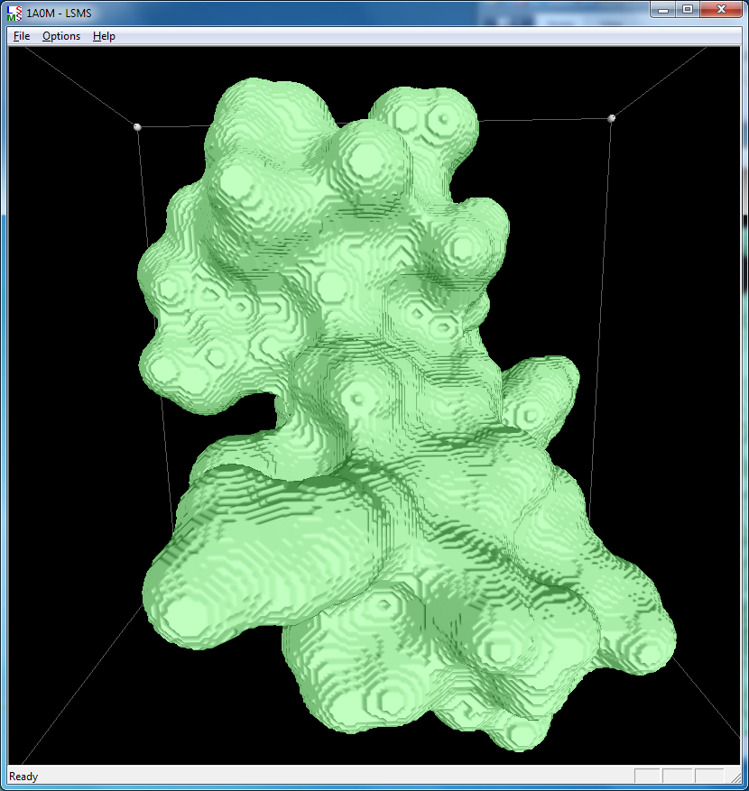
| 1a0m, 284 atoms, grid size 256, (quality 11) | 1f4h, 34,000 atoms, grid size 256, (quality 1.6) | 1jj2, 100,000 atoms, grid size 256, (quality 1.26) |
I think the Gaussian surfaces, sum of balls surface, and PyMol surfaces all look similar, so I'm guessing PyMol is the same kind of surface. Need to look at the PyMol source code to determine the exact method it uses. An hour perusal through PyMol 1.6 source code wasn't enough to figure out the surface calculation. It is C code, with 500 line routines with very sparse comments. It appeared that different surface calculation options were available. There are scans of distances to nearby atoms and a calculation of distance maps, and lots of references to "carving". With few comments and very long routines it is going to be a good deal of work to figure out this code.