
May 1, 2007
This tutorial focuses on display of volume data from single particle EM reconstructions. We'll look at maps of two conformations of human RNA polymerase II and a crystal structure of the homologous complex in yeast. This 12 protein complex walks along chromosome DNA making an RNA copy. The EM maps are described in the following article:
Kostek SA, Grob P, De Carlo S, Lipscomb JS, Garczarek F, Nogales E.
Molecular architecture and conformational flexibility of human RNA polymerase II.
Structure. 2006 Nov;14(11):1691-700.
Data sets and the most recent version of this tutorial (html, pdf) are online. The tutorial has been used with Chimera versions 1.2304, 1.2309, and 1.2382 and should work with more recent versions.
The 6 parts of the tutorial can be done in any order. They are ordered from simple to complex. Time required: ~2 hours.
|
|
|
|
|
|
|
|
|
|
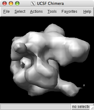
Use menu entry File / Open to open emd_1283.map found in the data directory of the downloaded tutorial files.
On a Mac with a one button mouse hold the option key down for middle mouse button, and the apple key down for right mouse button.
Holding the shift key down makes smaller motions for finer control.
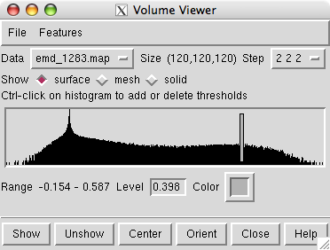
The volume viewer dialog indicates the map size is 120 by 120 by 120. The step size of 2 2 2 indicates that every other data plane is being used along the x, y and z axes.
Change the step size to 1 1 1 to show the full resolution data. The surface will appear smoother.
The volume dialog shows a histogram of the data values. Move the vertical bar on the histogram to change the contour level.
The displayed surface represents the positions in the map having value equal to the contour level. Higher contour level produces a smaller surface.
Press the square color button in the volume dialog to change the surface color. Move the black boxes on the color bars of the color dialog to adjust red, green and blue components of color.
Press the Opacity button on the color dialog and adjust the opacity (bottom color bar labeled with A) to make the surface transparent.
Use volume dialog menu entry
to display additional options and turn on option
This gives the surface a smoother appearance by moving each surface vertex a 0.3 of the way towards the average position of its neighbor vertices 2 times.
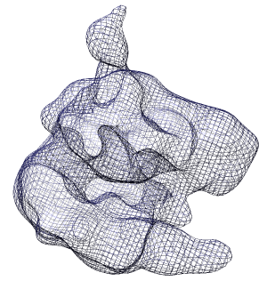
Click the Mesh switch on the second line of the volume dialog.
Click on the
option in the Features / Surface and Mesh Options panel. Turn off surface smoothing. In square mesh mode with no smoothing the displayed mesh corresponds to the intersection of volume xy, yz and xz grid planes with the surface.
Click on
This enables antialiasing, a method for blurring the jagged pixel jumps on each line segment. Zoom in close to see the effect. With some graphics cards this may not change the appearance.
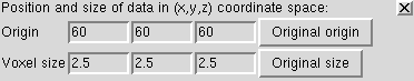
Use volume menu entry
The voxel size gives the spacing between grid planes along x, y and z axes. For this map it is 2.5 Angstroms.
Often a map file will not contain the grid plane spacing and in those cases you can enter correct values here. Correct scale is needed for fitting atomic models.
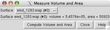
Open emd_1283.map if it is not already opened. We will set the contour level so that the surface encloses the estimated volume of the 12 protein hRNAPII complex of approximately 544,000 Å3. The estimate uses 1.21 Å3 per dalton (Harpaz 1994) and molecular weight of 450 kDa.
Use menu entry
and press the Compute Volume and Area button. Adjust the contour level and recompute the volume to find the contour level giving the desired volume. In Chimera version 1.2382 and newer the enclosed volume will automatically update as you vary the contour level.
|
|
|
|
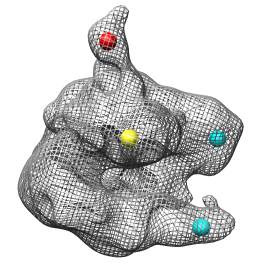
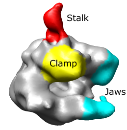
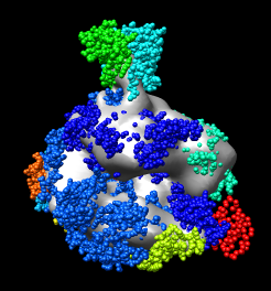
The RNA polymerase complex has features called the "stalk", "clamp" and "jaws". We will color and label these parts of the map. Open emd_1283.map if it is not already opened.
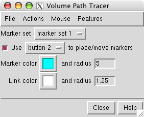
First we will place markers and then color the map near those markers. Open the marker placement dialog with menu entry
Click on the map stalk with the middle mouse button to place a marker. Display the map as a mesh so the marker can be seen within the surface.
When a marker is placed its z position (perpendicular to the screen) is the first density maximum along the line of sight through the mouse position.
To delete a marker first select it by holding the ctrl key and clicking on it with the left mouse button. Then use path tracer dialog menu entry
You can select more than one marker by dragging a box while holding the ctrl key. Or you can hold the shift and ctrl keys to to add individual markers to the selection.
When you place additional markers they will be connected by cylindrical links. To delete a link first select it (ctrl left mouse button) then use path tracer dialog menu entry
To disable automatic connection of markers use menu entry
To enable moving markers use menu entry
Then use the the middle mouse button to drag the markers. To move them perpendicular to the screen hold the shift key while dragging.
Change the color of the marker by selecting it (ctrl left mouse button) and pressing the square Marker color button in the path tracer dialog.
Increase the sphere radius of a selected marker to 5 Angstroms by typing 5 in the marker radius entry and pressing the Return key.
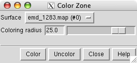
To color the map surface near the markers use main menu entry
The color zone tool colors the surface within a specified radius of the markers to match the color of the nearest marker.
Select all of the markers by holding the ctrl key and dragging a box around all of them with the left mouse button. Press the Color button on the color zone dialog and move the radius slider to about 25 Angstroms. Change the map display to surface in the volume dialog.
To reenable moving maps with the middle mouse button turn off
in the path tracer dialog.
To place text labels on the color regions use main menu entry
Click in the graphics window and then type to create a text label. Labels can be repositioned with the mouse. They can be deleted using the 2D label dialog. These 2D labels do not move when the map is rotated. They are primarily used for making figures with menu entry
To reenable rotating maps with the left mouse button close the 2D label dialog.
The human RNA polymerase II was seen in two conformations. We will now look at the difference between the maps by morphing one map into the other.
Open emd_1283.map if it is not already opened. Open the second map emd_1284.map using menu entry File / Open. It is useful to make this map a different color, and display one map in mesh style and the other in surface style to see both clearly.
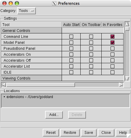
You have to tell Chimera where to find the map morphing tool. It is a plug-in that is not distributed with Chimera but is included in the extensions directory of the downloaded tutorial files.
Use menu entry
select
and press the button
near the bottom of the preferences dialog and choose the directory called
that contains a directory called MorphMap. You add the extensions directory and Chimera finds all plug-ins in that directory.
If you do not have the morph map tool you can obtain it online from the Chimera experimental features web page.
|
|
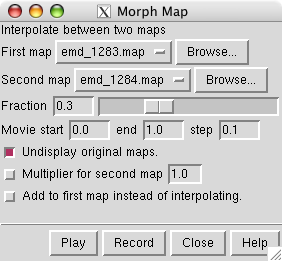
To display the morph map dialog use main menu entry
Choose emd_1283.map as the first map and emd_1284.map as the second map, and press
at the bottom of the dialog.
The two maps are not identically normalized, they do not enclose the same volume at the same contour level. A contour level of 0.339 gives volume 540,000 Å3 for map emd_1283 but a lower contour level of 0.326 is needed for map emd_1284. To morph between equal volume end-points turn on the option
using 1.04 (= 0.339 / 0.326) as the multiplier for the second map.
The morph animation can be saved in several formats (Quicktime, MPEG-2, ...). Press the Record button to save the animation.
You may wish to decrease the step value to create a smoother animation. A step of 0.1 creates 20 frames in going from an interpolation parameter of 0 (first map shown) to 1 (second map shown) and back to 0. A step of 0.02 would produce an animation of 100 frames.
|
|
|
|
|
We will fit a crystal structure of yeast RNA polymerase II into the EM map of the human complex. Currently no crystal structure of the human complex is available.
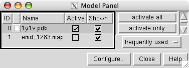
Close your current Chimera models using menu entry
and open 1y1v.pdb and emd_1283.map.
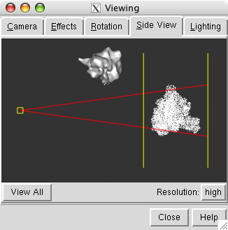
The PDB model and map are far apart. To see both use menu entry
The side view window shows the models from the side (perpendicular to the view in the main window). Move the vertical yellow lines which represent clip planes so both the map and model lie between them. The yellow square on the left in the side view represents your eye. Move it left or right to zoom out or in.
To move the model closer to the map use menu entry
Lock the map position by clicking off the checkbutton in the Active column next to emd_1283.map. Then move the PDB model so that it overlaps the map. Then turn back on the Active checkbutton so the map and model can both be moved.
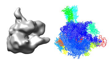
To color the distinct proteins of the PDB model first display the Chimera command line using menu entry
then type the command
rainbow chain
in the entry field at the bottom of the Chimera graphics window.
Orient the map so its stalk is pointing up and you look into the cleft. Then lock the map position using the model panel dialog and rotate the PDB model so it is similarly oriented and superimposed on the map.
Note that ctrl middle mouse button moves the model perpendicular to the screen.
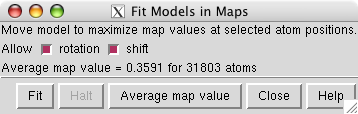
Do a computational optimization of the fit of the model in the map using menu entry
Select all atoms by dragging a box around them using the ctrl key and the left mouse button. Then press the Fit button. After a few seconds of steepest descent optimization the PDB model is moved to its optimized position. Sometimes pressing Fit again will improve the fit further.
Unselect all atoms by clicking with ctrl left mouse button on the black background in the Chimera graphics window.
If you have fast graphics you can display atoms as spheres using menu entry
If rotating the map and model is too slow return to the default display style with
An alternate approach to fitting is to create a theoretical density for the PDB model at the experimental map resolution (22 Å) using the pdb2mrc program in the EMAN package. Then fit that map into the experimental map. Chimera version 1.2318 and newer versions can optimize the fit of one density map in another map using
and report the correlation.
|
|
Chain S of 1y1v shown in red (when colored with command rainbow chain) is an elongation factor that was not present in the EM sample. To delete it, hold the ctrl key and click on a single red atom to select it. Then press the up arrow key to extend that selection to all of chain S. Then use menu entry
A crystal structure is available for the human RNA polymerase II stalk that we will compare to the yeast stalk. Open 2c35.pdb, color its chains with Chimera command
rainbow chain
and delete all chains except A and B with command
delete #2:.C-V
(delete model number 2 chains C through V). The asymmetric unit of this crystal structure contained four copies of the stalk dimer, three of which you just deleted (chains C,D,E,F,G,H), plus 4 chains (S,T,U,V) containing water molecules.
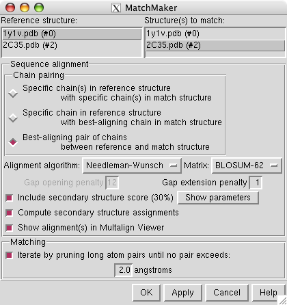
To align the human stalk (2c35) with the yeast stalk (1y1v) use menu entry
select reference structure 1y1v and structure to match 2c35 and press Apply. This will do a sequence-based structure alignment, move the human stalk model to align it with the yeast model, and display a sequence alignment of the best matching pair of chains.
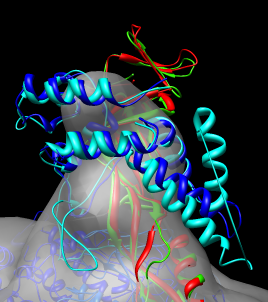
Show the models with ribbons using the two menu entries
and for better looking ribbons
While the structures are very similar notice that one alpha helix of the yeast stalk (cyan) that is far out of the density is not part of the human structure (dark blue).
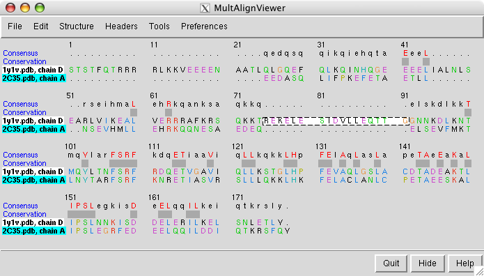
The sequence alignment shown by the match maker tool is for the human and yeast chains that matched best (B and G). To look at a sequence alignment of the other pair of chains where yeast has an extra helix use the match maker chain pairing option
choose 1y1v chain D as the match maker reference chain and press Ok.
Dragging a box around the yeast sequence insertion (positions 75 - 91) in the MultAlignViewer sequence window will highlight the corresponding residues (the extra helix) in the graphics windows.
For a closer view of this helix, select it and use menu entry
to zoom in, set the near and far clip planes, and set the center of rotation about those atoms.
The data sets for this tutorial are included in the data directory of the tutorial files (chimera-tutorial.zip), or can be obtained from public databases:
The map files will have to be uncompressed using command-line program gunzip on Linux or Stuffit Expander on Mac OS X. On Windows XP you have to install decompression software such as Win-GZ.
For more information about Chimera volume display capabilities look at the
Also see additional tutorials, experimental features, image gallery, animations, examples, user's guide, and the Chimera home page http://www.cgl.ucsf.edu/chimera.