The purpose of this exercise is to get familiar with Chimera features for density map display, and display of Protein Data Bank (PDB) models.
This tutorial is based on Chimera version 1.2105 (March 2005). Some features described may have changed in more recent Chimera versions.
This tutorial uses a PDB file and a density map that you can download from this web site (1OEL.pdb, emd_1080.map) or from the PDB and Macromolecular Structure Database web sites (1OEL.pdb, emd_1080.map).
Followed by more advanced features:
And miscellaneous topics
On Linux run the executable "chimera" in the bin directory of your Chimera installation. If Chimera is installed in /usr/local/chimera, then you run /usr/local/chimera/bin/chimera from a shell.
On Windows start Chimera by double clicking the Chimera icon in the directory called bin in your Chimera installation. If Chimera is installed in \Program Files then the executable will be found in directory \Program Files\Chimera\bin.
On Mac start the Apple X server found in /Applications/Utilities/X11. Then double click the Chimera application to start. The X server is not installed in Mac OS 10.3 by default and if you do not have it you can download it from the Apple web site. It is necessary for running Chimera on the Mac. NB: Chimera for Mac OS X now uses the native Apple interface rather than X11.
Use the Chimera File / Open dialog to open emd_1080.map. In the File Open dialog you should change the File Type to All (guess type). Initially it is set to only show Protein Data Bank files (*.pdb).
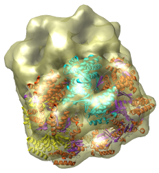
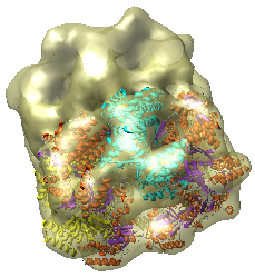
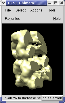
This is a single particle reconstruction of GroEL determined by Steve Ludtke using EMAN software. GroEL is a cylindrical 14-mer that refolds misfolded proteins in its interior cavity. This density map and others are available from the EM database at the Macromolecular Structure Database.
This GroEL map has 11.5 angstrom resolution. Another map determined by Steve having 6 angstrom resolution is also available. We'll use the lower resolution map because it is easier to see the main features.
Dragging the mouse in the graphics window lets you rotate, translate, and zoom in on the map.
On a Mac with a one button mouse, hold down the Option key to get middle mouse button behaviour, or the Command key to get right mouse button behaviour.
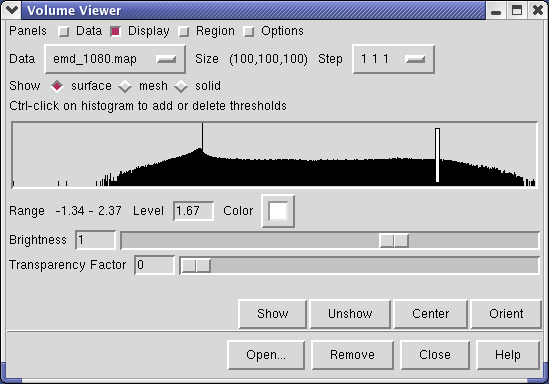
Controls for display of volume data (ie density maps) are in the Volume Viewer dialog that was displayed when you opened the file. If you close this dialog it can be shown again with menu entry Tools / Volumes / Volume Viewer.
The center histogram shows the distribution of data values in the density map. The range of data values (-1.34 to 2.37) is shown below the histogram. The white vertical bar on the histogram shows the contouring threshold. Drag this bar with the mouse to change the contour level. The numeric value of the contour level is shown below the histogram in the entry field. Contour levels can be typed in instead of being set with the mouse.
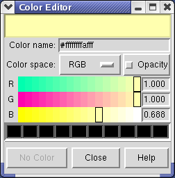
Clicking on the white square with the wide raised border below the histogram shows a Color Editor dialog. The square button, called a Color Well, is used in many Chimera dialogs to choose colors and shows the current color in the center. Change the density map color by clicking on the color bars in the Color Editor dialog. You can close the dialog when you are done.
Above the histogram is a radio button where you can choose mesh display style. This shows the surface as a mesh made up of triangles. You may need to zoom in to see the small triangles.
Near the top of the dialog the data size, 100 by 100 by 100, is shown. The Step menu allows you to subsample the data. For example, a step of 2 2 2, means to use every other density value along each of the 3 axes. Subsampling is useful with large maps to speed up moving and recontouring.
The outline box shows the bounds of the data set. You can hide the outline box by clicking the Options checkbutton on the right side of the top line of the Volume Viewer dialog. This displays a panel of options and the first one Show outline box... can be switched off. Clicking the Options checkbutton again hides the long panel of options.
To make the density map display brighter use menu entry Tools / Viewing Parameters / Effects and switch off Depth cueing in the Viewing dialog. Depth cueing makes objects appear dimmer the further they are away from you. This will be discussed more in the section on tricks for better images It is a good idea to close Chimera dialogs when you are done so your whole screen does not become covered with dialogs.
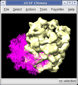
We now look at an atomic model of GroEL determined by x-ray crystallography, and how this can be aligned with the density map.
Use File / Open to open Protein Data Bank model 1OEL.pdb. It is in the same directory as the density map. The atomic model of one half of GroEL will be shown shifted to one side of the density map.
We'll look at methods of atomic model display now. First hide the density map using menu entry Favorites / Model Panel and switching off the checkbutton in the Shown column for emd_1080.map.

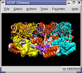
To show a ribbon display of the model use menu entry Actions / Ribbon / show. To hide the original all-atom display use menu entry Actions / Atom+Bonds / hide. Zooming in shows a flat ribbon. To make the ribbon have an oval cross-section use Actions / Ribbon / round.
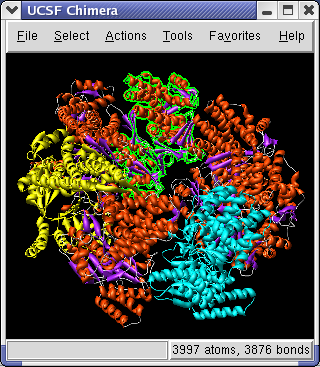
To color the alpha helices, beta sheets and turns of the ribbon using separate colors, click on the 1OEL.pdb line in the Model Panel dialog and then press the Color by SS... button in the righthand column of that dialog. The SS is short for secondary structure. Press the OK button on the color secondary structure dialog to use the default colors.
To color one of the 7 proteins in this model differently, select a single residue using the mouse.
The selected residue will be highlighted with a green outline. It may be hard to see since it is small. Pressing the up arrow key on the keyboard (the one used for moving up one line in a text editor) will extend the selection to the entire chain containing that residue. Then use menu entry Actions / Color / cyan to color the selected chain.
To select a chain by its PDB identifier, use menu Select / Chain which contains entries A, B, C, D, E, F, G corresponding to the 7 chains in PDB model 1OEL. Choose any chain from the menu to select it.
To hide the selected chain use Actions / Ribbon / hide. You use Ribbon / hide instead of Atoms+Bonds / hide because the chain is displayed as a ribbon. The hide menu entries for the two styles are separate because you can have both ribbon and atoms/bonds showing at the same time.
To select multiple chains, select a residue from one chain with Ctrl left mouse button. Then select a residue in another chain with Shift Ctrl left mouse button. Adding the Shift key extends the existing selection instead of replacing it. Then press the up arrow key to select both chains.
When an object is selected the model may not rotate smoothly because drawing the green outline around the object requires alot of computation. To clear the selection click Ctrl left mouse on empty space, or use menu entry Select / Clear Selection.
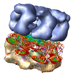
Now we will move the PDB model to align it with the density map.
Redisplay the density map using the Model Panel dialog (menu entry Favorites / Model Panel) by clicking the checkbutton in the Shown column next to emd_1080.map. Display the density map as a mesh using the Volume Viewer dialog (menu entry Tools / Volumes / Volume Viewer).
Rotate with the mouse so you are looking directly down the axis of GroEL cylinder with the 1OEL model near you.
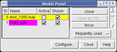
Now switch off the Active checkbutton next to emd_1080.map in the Model Panel dialog. This in the column before the Shown button and each model has a separate checkbutton. Active means that the model can be moved with the mouse. Now use the middle mouse button to drag the PDB model so that it is centered with the density map.
Once the PDB model is centered with the density map drag with the left mouse button near the edge of the graphics window to rotate the PDB model to match the shape of the density map. When you do a mouse rotation at the edge of the window, this rotates about the axis perpendicular to the screen. Using the mouse more towards the middle rotates the model about axes parallel to the screen as if you are grabbing the model. The boundary between these mouse rotation zones is not shown.
Turn on the Active button on the Model Panel for emd_1080.map so you can rotate both models at once and check the alignment from different view points.
If you accidentally rotate the PDB model so its axis is not parallel to the density map cylinder axis, use menu entry Tools / Utilities / Undo Move to bring them back to having parallel cylinder axes.
| File / Save Image... | Screen shot (jagged edges) |
|
|
|
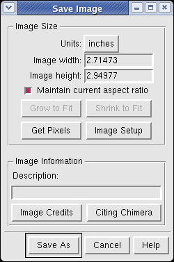
Use menu entry File / Save Image... and press the Save As button to save the graphics window image to a file. After the image is captured a dialog appears to choose the file name and format.
The Chimera dialogs will disappear and you will see magnified pieces of the image flash by in the graphics window. Chimera is capturing the image directly from the screen so no dialog should be placed on top of the Chimera window while the image is taken.
Using Chimera image saving will produce a higher quality image than taking a screen snapshot. The image is captured at a size 3 times larger than requested and then averaged down to the correct size. This is called supersampling. It reduces jagged edges.
You can make images larger than the screen for publications and posters. Type a new value into the dialog width or height entry fields and press the Enter key. You only need to enter one of the dimensions. When you press Enter the other will be calculated to maintain the aspect ratio, and the image will be captured. To change the pixels per inch press the Image Setup button.
If you want an image exactly the same number of pixels as the Chimera window on the screen, press the Get Pixels button. This fills in the exact size in pixels of the Chimera graphics window.
When making images sometimes you want the background to be white. Do this using menu entries Actions / Color / background followed by Actions / Color / white.
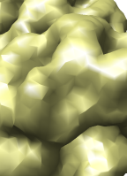
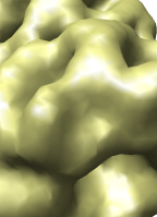
| Smoothing off. | Smoothing on. |
| 
|
Zooming in on the surface you can see facets from the triangles (use surface display style). To reduce these you can turn on the surface smoothing. Click the Options checkbutton at the top of the Volume Viewer dialog and check the Surface smoothing iterations ... checkbutton, the last entry in the options panel. The list of options is so long it may go off the bottom of your screen. You may need to hide the Display panel by unchecking the Display checkbutton at the top of the Volume Viewer dialog to see the full list of options.
You can leave this option on -- its only serious drawback is that it can slow down recontouring the surface. To have make your changed Volume Viewer settings the defaults for future Chimera sessions press the Save default dialog settings button at the bottom of the Options panel.
Chimera settings are saved in a hidden directory called .chimera in your home directory in a file called preferences.
Chimera dims parts of the scene that are further from you to give a sense of depth. This feature can be turned on and off using menu entry Tools / Viewing Parameters / Effects.
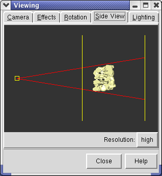
The dimming occurs between the near and far clip planes. The clip planes can be adjusted using menu entry Tools / Viewing Parameters / Side View. The Side View window displays the open models as seen from the side. Two vertical yellow lines indicate the front and back clip planes. The left line is the front clip plane. If you drag the front clip plane (yellow vertical line) towards the models with the mouse you will see the brightness in the main graphics window increase (provided depth cueing is turned on). If you move the front clip plane so it intersects the models, you will see the surface cut in the main graphics window.
The small yellow box at the left in the side view is your eye position. You can drag this left or right to zoom in and out.
The Tools / Viewing Parameters / Lighting menu entry lets you move the 2 Chimera lights. The key light provides the main illumination of your models while the fill light.is intended to fill in dark areas.
You can control how shiny the models appear using menu entry Tools / Viewing Parameters / Shininess Control. The shininess parameter effects the size of specular highlights. Specular highlights are the white lighting spots on the model. The brightness parameter just effects the brightness of the highlights, not the whole surface.
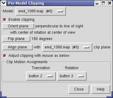
The Tools / Graphics / Per-Model Clipping menu entry lets you slice through surfaces (and protein models). Set the model to emd_1080.map and turn on the Enable clipping switch in the dialog that is shown. Then rotate the density map to see the cut.
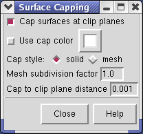
The cut surface is visually confusing because you see inside of the surface. Use the Tools / Graphics / Surface Capping menu entry and switch on Cap surfaces at clip planes. This will cap the hole where the surface was cut.
To move the cut plane, also called the clipping plane, switch on the Adjust clipping with mouse... switch in the Per-Model Clipping dialog. Then drag the clip plane with the middle mouse button or rotate it with the right mouse button. Turn off the Adjust clipping with mouse... switch to restore the mouse buttons their normal behaviour of translating models and zooming.
| 
|
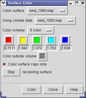
The density map values vary across the clipped capped surface. The variation can be shown by coloring the cap using Tools / Volumes / Surface Color. Change the Color scheme in the Surface Color dialog to be 5 color. (The 3 color color scheme is intended for display of electrostatic potentials.) To only color the cap switch on Color surface caps only. Then press the Color button at the bottom of the dialog.
When you move the clip plane, the coloring will be automatically updated.
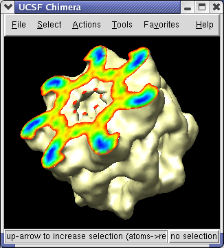
To clip the GroEL density perpendicular to the cylindrical axis, first press the Orient button on at the bottom of the Volume Viewer dialog, then press the Orient plane perpendicular to line of sight button on the Per-Model Clipping dialog. The Orient button on the volume dialog rotates the density map back to the original orientation when the file was first opened (z-axis perpendicular to screen). After orienting the plane try moving it with the middle mouse button.
If you change the contouring threshold in the Volume Viewer dialog by dragging the marker on the histogram, the colors on the capped surface will change by small amounts. Ideally they should not change and the problem is that the volume data is not being sampled at enough points on the cut surface. You can see the sampling by switching Cap style to mesh in the Surface Capping dialog. The mesh switch in the Surface Capping dialog effects just the cap, while the mesh switch in the Volume Viewer dialog applies to just the contour surface. Increasing the Mesh subdivision factor in the Surface Capping dialog to 2.0 (press Enter after changing the number for change to take effect) will cause cap vertices to be more closely spaced by a factor of 2. Moving the contour threshold then produces very little artifactual color variation, but updates are slower.
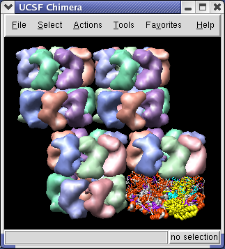
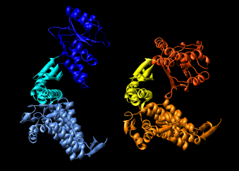
The 1OEL crystal structure has only one of the two 7 protein rings in its asymmetric unit. GroEL has two such rings stacked. The full GroEL can be seen by looking at the crystal unit cell.
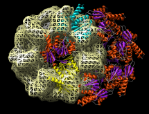
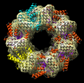
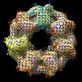
Use menu entry Tools / Multiscale / Multiscale Models and near the bottom of the Multiscale dialog choose Crystal unit cell for the Multimer type, and press the Make Models button.
The Multiscale dialog makes copies of PDB chains using symmetry matrices. It displays the copies as low resolution surfaces. Each of the 7 chains of a ring is given a different color.
You will see 4 GroEL barrels. Each barrel consists of two rings of PDB model 1OEL stacked to form a cylinder.
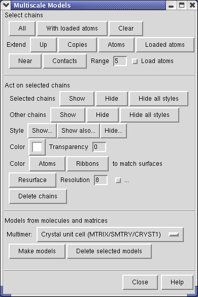
You can select individual surfaces using Ctrl left mouse button and change their color with the Color Well button in the middle of the Multiscale dialog. If you select a surface and then press the Copies button near the top of the Multiscale dialog it will extend the selection to all copies of that chain.
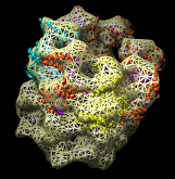
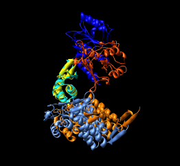
Press the With loaded atoms button in the selection pane at the top of the Multiscale dialog, and towards the middle of the dialog use the Style Show... button which pops up a menu and select Ribbon. This shows your original copy of 1OEL.
Delete the 3 extra copies of the GroEL barrel by selecting each barrel with the mouse and pressing the Delete Chains button in the Multiscale dialog. You can select a barrel with the mouse using Ctrl left mouse button and dragging a box around it. This selects everything in the rectangle you drag out (highlighted in green). To avoid selecting molecules you do not wish to delete it is best to drag a small box -- only a piece of each molecule need be in the box to be selected. Even if a molecule is hidden from view behind another one, it will be selected if it partially lies in the box you draw.
The 1OEL PDB model is a crystal structure that has a B-factor associated with each atom that indicates how well localized the atom is in the x-ray density. To display the B-factor using ribbon thickness select the 1OEL.pdb line in the Model Panel and press the Render by attribute button in the right column of that dialog. It will take several seconds to scan the attributes of this large (27,000 atom) structure.
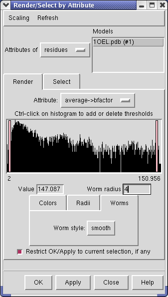
Choose Attributes of residues in the Render by attribute dialog, choose Attribute to be average -> b-factor, then switch to the Worms tab, and press Apply.
The ribbon thickness now corresponds to average residue b-factor value. The low b-factor face of 1OEL lie at the interface between the two 7-mer rings, and the high b-factor face is at the end of the barrel.
If you had a chain selected, only that chain shows the thickness variation. If you clear the selection (Ctrl click on empty space, or menu entry Select / Clear Selection) and press Apply again all chains will show b-factor.
The Render by attribute dialog shows a histogram of the b-factor values. Vertical bars on the histogram mark B-factor values which have a specified thickness. For b-factor values between the bars the ribbon radius is linearly interpolated using the values defined for the bars.
Clicking on a histogram bar shows the corresponding ribbon thickness in the Worm radius entry field below. The bars can be moved and radii changed. Unlike the Volume Viewer dialog where moving the histogram bar causes an immediately updated display, here you need to press Apply to see the effect of your change.
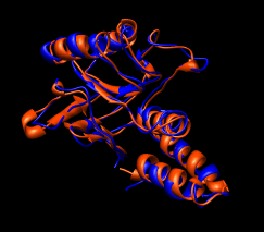
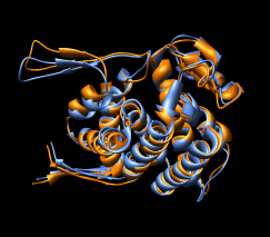
GroEL adopts different conformations and our hand alignment of PDB model 1OEL and density map emd_1080 is only a first step in comparing this crystal and single particle EM data. The GroEL monomer has 3 domains that can assume different orientations relative to one another. A next step would be to computationally fit the individual protein domains into the EM map.
Chimera does not compute optimal positioning of PDB models or domains in density maps. You would need to use other software to do that.
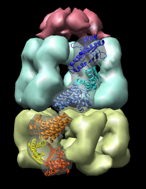
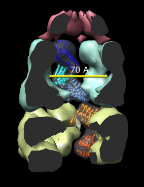
Here are a series of Chimera images showing the 3 domains of the GroEL monomer. Two monomers in PDB model 1AON having identical amino acid sequence but different conformations are compared.

Several steps were used to produce these images that we will not describe here.
Some of the tools used to make these images are:
You can put buttons for frequently use Tools on the left side of the main Chimera window using Favorites / Preferences....
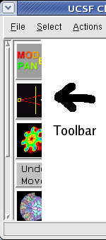
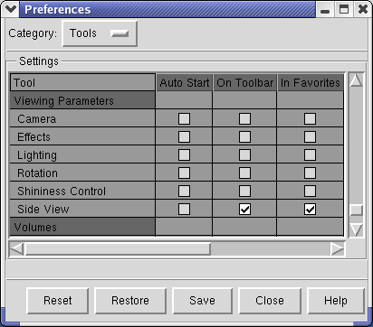
The Preferences dialog has several categories of preferences. Choose the Tools category. The entries in this list of tools are exactly those in the Tools menu, in the same order. Check buttons in the second column of the scrollable list of tools to put a button that invokes that menu entry on the Toolbar at left side of the main window. For example, check Inspectors / Model Panel and Viewing Parameters / Side View.
If you want these buttons to appear every time you start Chimera, press the Save button at the bottom of the Preferences dialog.
Pressing the Help button at the bottom of any Chimera dialog will show the appropriate section of the Chimera manual (included with the Chimera distribution) in your web browser. Almost all Chimera dialogs have these help buttons. The user manual documentation is very thorough and worth looking at. Also look at the Help menu on the main window.
You can save your Chimera session with File / Save Session As.... Later you can restart Chimera and use File / Restore Session to redisplay your models. This will save the PDB models, Multiscale surfaces, density map display settings, colorings, background color, and many other attributes. It does not save all aspects of the session. The surface clipping, capping and coloring shown before are not saved in our current version, but may be in future releases.
The session is saved as a Python file (.py file suffix). It saves a copy of the PDB data but does not copy the density map data. For density maps it saves the path to the original file. For large PDB models such as 1OEL (27,000 atoms) saving and restoring the session can take a few minutes.
Chimera has many tools not explored in this tutorial. Most are for analyzing and comparing protein structures and sequences.
More tutorials can be found in the Chimera User's Guide using the Chimera Help / Tutorials menu entry, or possibly more recent ones on the Chimera web site http://www.cgl.ucsf.edu/chimera in the User's Guide.