open 4191 from emdb
or smaller middle 1/3 of tomogram for faster download (25 Mbytes)
open https://www.rbvi.ucsf.edu/chimerax/data/rml-sep2019/data/emdb_4191_small.mrc
or if previous site is down
open http://sonic.net/~goddard/rml-sep2019/data/emdb_4191_small.mrc
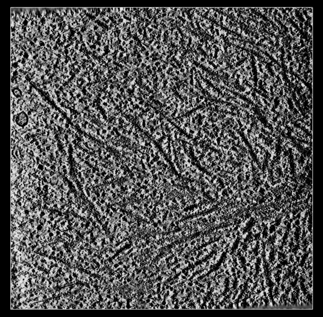
a) Tomogram EMDB 4191 is 240 Mbytes and can be slow to download.
b) Size 926 x 926 x 71 grid points, 32-bit float values reported in Log.
c) ChimeraX caches fetched data under folder ~/Download/ChimeraX
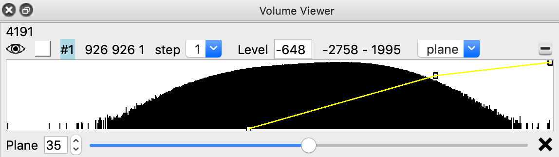
volume scale #1 factor -1
Close original map
close #1
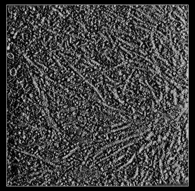
a) Tomogram lower map values correspond to higher density.
b) Map values represent how much of the electron beam passed through the sample and hit the detector.
c) It is useful for visualization to make high values correspond to high density by inverting values.
d) The "volume scale" command creates a copy of the map in memory. It does not modify the original map.
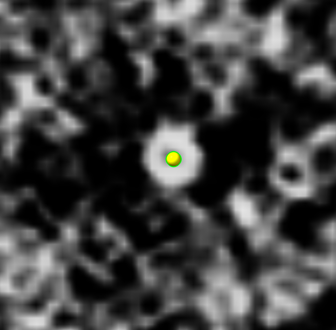
Marking proteasomes
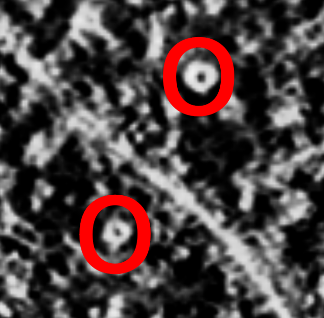
Right click (Cmd+click on Mac) to place markers on proteasomes.
volume box #2 center #1 isize 32
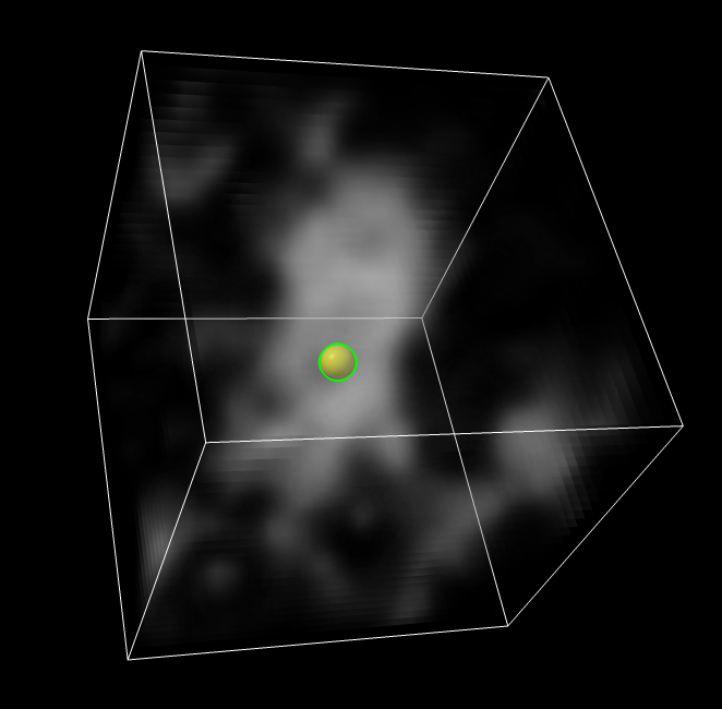
save ~/Desktop/proteasome1.mrc model #3
To save markers to an XML text file
save ~/Desktop/proteasomes.cmm model #1
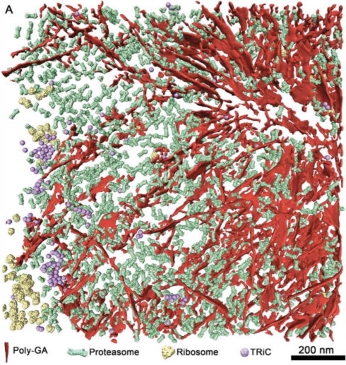
In article Guo Q, Cell Feb 2018 10000 proteasomes in 9 tomograms found with custom MATLAB and TOM toolbox template matching algorithms.
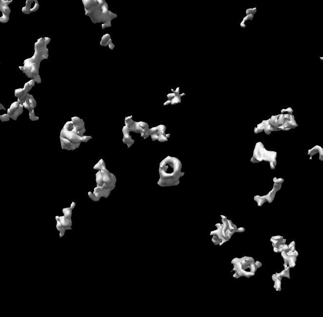
Surface depictions
volume #2 style surface level 780
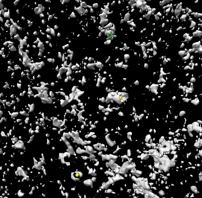
surface dust #2 size 200
Click proteasome surfaces to measure size.
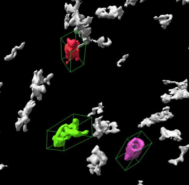
a) Picked blob Log output.
volume = 7.4896e+05
area = 87962
size = 325.01 111.15 115.29
b) Blob mouse mode draws a box aligned with the principle axes of inertia and reports lengths along those axes.
c) Blob coloring is lost when surface level is changed.
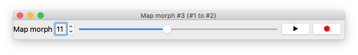
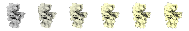
Comparing subtomogram maps by morphing
Guo Q, Cell Feb 2018 averaged proteasomes from tomogram with 4 different shapes. Two conformations were degrading ubiquitinated protein. We will look at two "ground state" conformations with no substrate.
close
Open two subtomogram average maps
open 3913 from emdb
open 3916 from emdb
volume morph #1,2
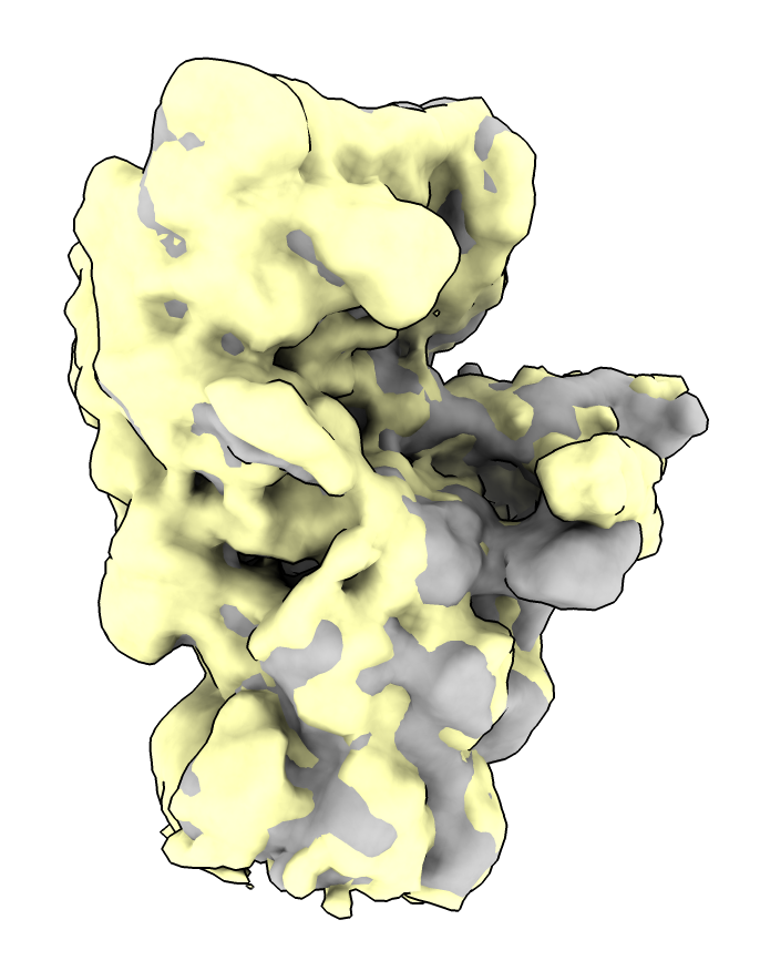
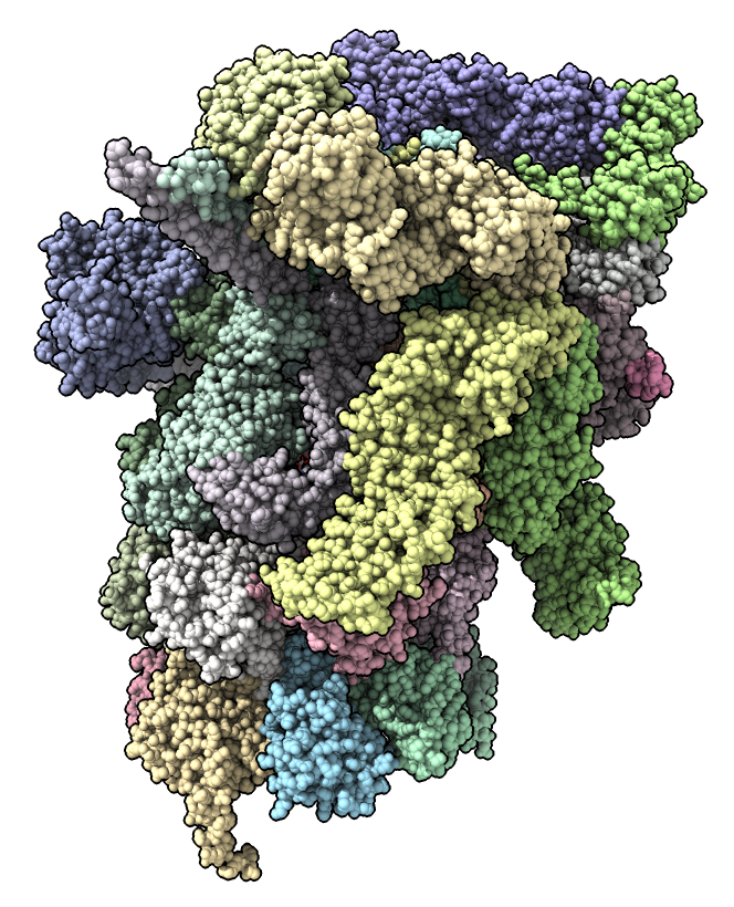
Fitting atomic models
Guo Q, Cell Feb 2018 fit atomic structures of proteasomes degrading substrate or not bound to substrate to infer the state of the proteasomes and concluded many proteasomes are stalled, unable to digest the poly Gly-Ala fibrils.
We will fit an atomic model of a proteasome into one of their subtomogram average proteasome maps at 12 Angstroms resolution.
close
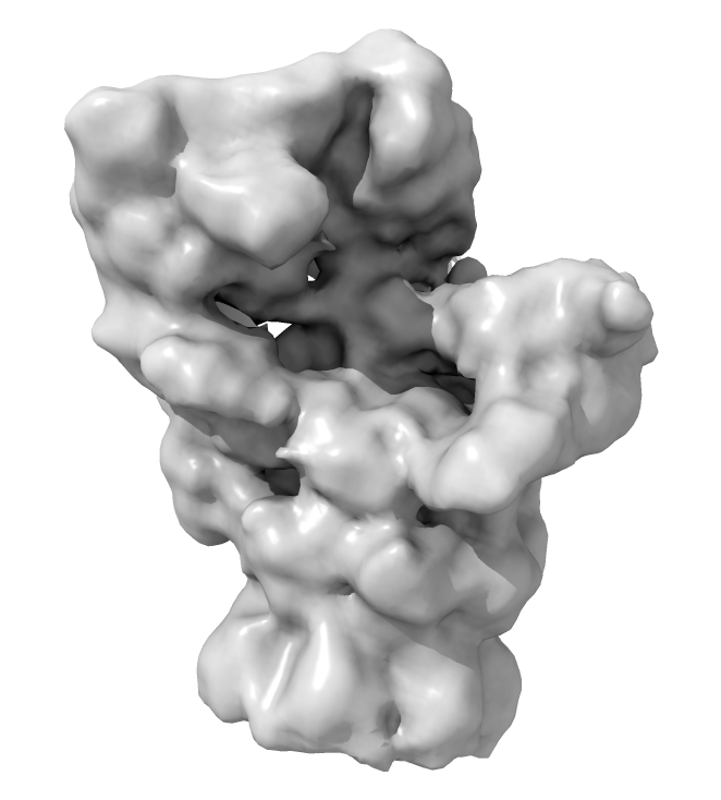
Open subtomogram average map
open 3913 from emdb
open 5mpc
Center view
view

Delete extra proteins from atomic model.
del /a-n,X
select #2
Use Move Model mouse mode from Right Mouse toolbar.
a) Hold the shift key to rotate, no-shift to translate.
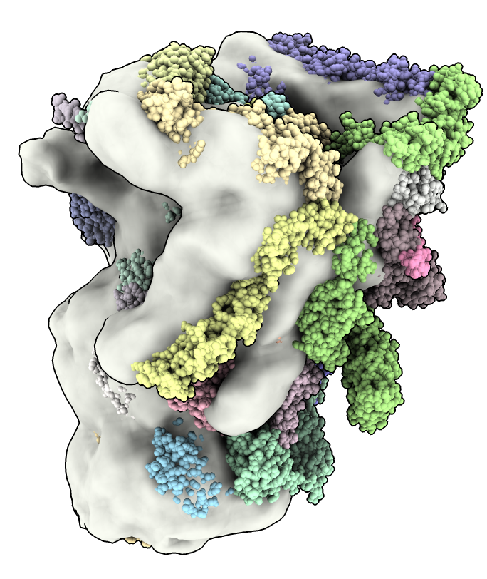
fit #2 in #1
Make surface transparent with Map toolbar Transparent button, or command
transparency #1 30
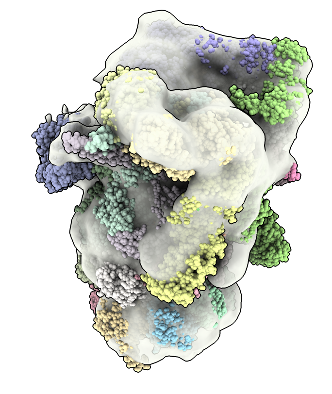
a) Guo's proteasome maps are half-proteasomes. The proteasome is a cylinder made of two rings and a lid complex on either end. A half proteasome has one ring and a lid.
b) The fitmap command does a rigid rotation and translation to optimize the position of an atomic model in a map.
c) To rotate with mouse or trackpad about the axis perpendicular to the screen click near the edge of the graphics window and drag.