


clusterMaker2: Creating and Visualizing Cytoscape Clusters
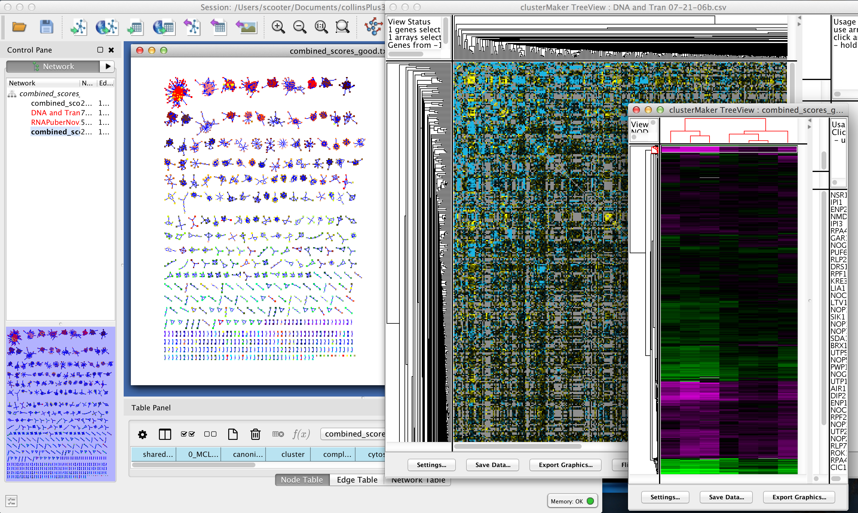
Figure 1. clusterMaker2 in action. In this screenshot, the yeast protein-protein interaction network from Collins, et al. (2007a) has been clustered using MCL. A yeast expression data set from Gasch, et al. has been imported into the PPI data, and a yeast genetic interaction dataset from Collins, et al. (2007b) has been imported as a separate network. All of the networks share node identifiers so they may be linked. The genetic interaction network and the expression data set are shown as heatmaps.
UCSF clusterMaker2 is a Cytoscape app that unifies different clustering, filtering, ranking, dimensionality reduction algorithms along with appropriate visualizations into a single interface. Current clustering algorithms include hierarchical, k-medoid, AutoSOME, k-means, HOPACH, and PAM for clustering expression or genetic data; and MCL, transitivity clustering, affinity propagation, MCODE, community clustering (GLAY), SCPS, and AutoSOME for partitioning networks based on similarity or distance values. In addition to the latter group, remotely running algorithms have been implemented in the newest release including Leiden, Infomap, Fast Greedy, Leading Eigenvector, Label Propagation and Multilevel clustering. Furthermore, fuzzy C-Means and a new "fuzzyfier" algorithm have been added to provide support for fuzzy partitioning of networks. Network partitioning clusters may also be refined by post-cluster filtering algiorithms. clusterMaker2 provides the ability to create a correlation network based on creating a distance matrix from a list of attributes and creating a "clustering" by assigning the connected components of a network to a cluster. Hierarchical, k-medoid, AutoSOME, and k-means clusters may be displayed as hierarchical groups of nodes or as heat maps. All network partitioning cluster algorithms create collapsible groups to allow interactive exploration of the putative clusters within the Cytoscape network, and results may also be shown as a separate network containing only the intra-cluster edges, or with inter-cluster edges added back.
In addition to the classical clustering algorithms discussed above, clusterMaker2 provides five algoririthms to rank clusters based on potentially orthogonal data (e.g. ranking the results of an MCL cluster based on expression data results), and dimensionality reduction approaches including Principal Component Analysis (PCA), Principal Coordinate Analysis (PCoA) and t-Distributed Stochastic Neighbor Embedding (tSNE) (hardcoded and remote implementations). clusterMaker2 also provides a selection of remotely calculated dimensionality reduction techniques namely Uniform Manifold Approximation and Projection (UMAP), Isomap, Locally Linear Embedding (LLE), Multidimensional Scaling (MDS) and Spectral Embedding.
clusterMaker2 requires version 3.8.0 or newer of Cytoscape and is available in the Cytoscape App Store.- Installation
- Starting ClusterMaker2
- Attribute Cluster Algorithms
- Network Cluster Algorithms
- Affinity Propagation
- Cluster "Fuzzifier"
- Connected Components
- Community Clustering (GLay)
- Fuzzy C-Means Clustering
- MCODE
- MCL
- SCPS (Spectral Clustering of Protein Sequences)
- Transitivity Clustering
- Leiden Clustering (remote)
- Infomap (remote)
- Fast Greedy (remote)
- Leading Eigenvector (remote)
- Label Propagation (remote)
- Multilevel Clustering (remote)
- Filtering Clusters
- Ranking Clusters
- Dimensionality Reduction
- Principal Components Analysis
- Principal Coordinates Analysis
- t-Distributed Stochastic Neighbor Embedding
- t-Distributed Stochastic Neighbor Embedding (remote)
- Uniform Manifold Approximation and Projection (remote)
- Isometric Mapping (remote)
- Locally Linear Embedding (remote)
- Multidimensional Scaling (remote)
- Spectral Embedding (remote)
- Visualizing Results
- Interaction
- Commands
- Acknowledgements
- References
1. Installation
clusterMaker2 is available through the Cytoscape App Store or by downloading the source directly from the RBVI git repository. To download clusterMaker2 using the App Store, you must be running Cytoscape 3.8.0 or newer. To install it, either launch Cytoscape 3.8.0 and then go to the App Store in your internet browser and search for "clusterMaker2". If you select the "clusterMaker2" button, you should get to the clusterMaker2 App page and the Install button should be available. Click on it and it will automatically install into Cytoscape. Alternatively, you can use the Apps→App Manager and search for clusterMaker2 and install it.
2. Starting ClusterMaker2
Once clusterMaker2 is installed, it will install four menu hierarchies under the Apps main menu: clusterMaker Cluster Attributes (Figure 2), clusterMaker Dimensionality Reduction (Figure 4), clusterMaker Filter Clusters (Figure 5), clusterMaker Ranking (Figure 6) and clusterMaker Visualizations (Figure 7).
Each of the supported clustering algorithm appears as a separate menu item underneath the clusterMaker menu. To cluster your data, simply select Apps→clusterMaker→algorithm, where algorithm is the clustering algorithm you wish to use. This will bring up the settings dialog for the selected algorithm.
There are three different types of clustering algorithms supported by clusterMaker2:
- Attribute Cluster Algorithms: a list of node attributes or a single edge attribute is chosen to perform the clustering. The normal visualization is some kind of heat map where the rows correspond to the nodes in the network. Selection of a row selects the corresponding node in the network. If an edge attribute is chosen, the columns also correspond to the nodes in the network and selection of cell in the heat map selects an edge in the network.
- Network Cluster Algorithms: an edge attribute is chosen to partition the network. Fuzzy cluster algorithms also partition the network but nodes are allowed to be in more than one cluster. The normal visualization is to create a new network from the clusters.
- Network Filter Algorithms: these are designed to be executed after a Network Cluster Algorithm has been run to refine the resulting partitioning.
The clusterMaker Dimensionality Reduction menu contains the dimensionality reduction algorithms available in clusterMaker2. When the dimensionality reduction algorithm is selected, a settings dialog for it opens.
The clusterMaker Ranking lists all the ranking options implemented in clusterMaker2. Each menu item is a different ranking algorithm that when selected will open a settings dialog.
The clusterMaker Visualization menu contains the visualization options, including showing a heat map of the data (without clustering), and options appropriate for displaying Hierarchical or k-Means clusters if either of those methods had been performed on the current network. Because information about clusters is saved in Cytoscape attributes, the JTree TreeView and JTree KnnView options will be available in a session that was saved after clustering.
Some of the network cluster algorithms as well as majority of the dimensionality reduction techniques have been implemented using an RESTful API. It allows sending the network data to a remote server to be calculated and receiving the results back to the clusterMaker2 client. If the server does not respond in maximum of 20 seconds, the job moves to be executed asynchronously in the background. clusterMaker2 uses the algorithms on scikit-learn (https://scikit-learn.org/stable/modules/classes.html) API and classes in cytoscape.jobs package (http://code.cytoscape.org/javadoc/3.8.0/org/cytoscape/jobs/package-summary.html).
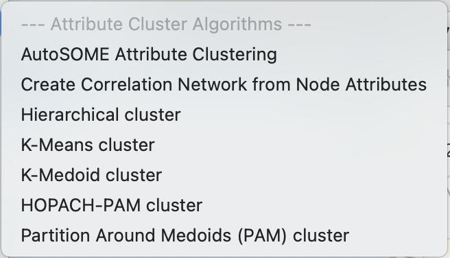
Figure 2. clusterMaker2 clusterMaker Cluster Attributes menu.
Figure 3. clusterMaker2 clusterMaker Cluster Networks menu.
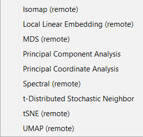
Figure 4. clusterMaker2 clusterMaker Dimensionality Reduction menu.
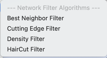
Figure 5. clusterMaker2 clusterMaker Filter Clusters menu.
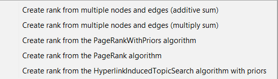
Figure 6. clusterMaker2 clusterMaker Ranking menu.

Figure 7. clusterMaker2 clusterMaker Visualizations menu.
3. Attribute Cluster Algorithms
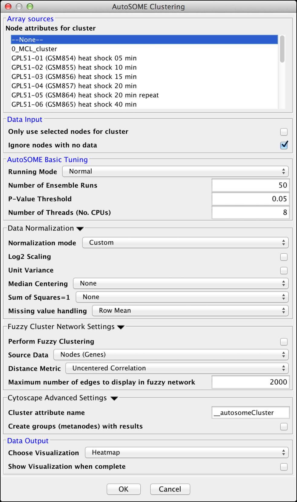
Figure 8. clusterMaker2 AutoSOME cluster dialog.
3.1 AutoSOME
AutoSOME clustering is the one cluster algorithm that functions both as an attribute cluster algorithm as well as a network cluster algorithm. The AutoSOME algorithm revolves around the use of a Self-Organizing Map (SOM). Unsupervised training of the SOM produces a low-dimensional reprentation of input space. In AutoSOME, that dimensionally reduced spaced is compresed into a 2D representation of similarities between neighboring nodes across the SOM network. These nodes are further distorted in 2D space based on their density of similarity to each other.Afterwards, a minimum spanning tree is built from rescaled node coordinates. Monte-Carlo sampling is used to calculate p-values for all edges in the tree. Edges below an inputed P-value Threshold are then deleted, leaving behind the clustering results. AutoSOME clustering may be repeated multiple times to minimize stochastic-based output variation. The clustering results stabilize at maximum quality with an increasing Number of Ensemble Runs, which is one of the input parameters. Statistically, 25-50 ensemble runs is enough to generate stable clustering.
Array Sources
- Node attributes for cluster:
- This area contains the list of all numeric node and edge attributes that can be used for hierarchical clustering. At least one edge attribute or one or more node attributes must be selected to perform the clustering. If an edge attribute is selected, the resulting matrix will be symmetric across the diagonal with nodes on both columns and rows. If multiple node attributes are selected, the attributes will define columns and the nodes will be the rows.
Data Input
- Only use selected nodes/edges for cluster:
- Under certain circumstances, it may be desirable to cluster only a subset of the nodes in the network. Checking this box limits all of the clustering calculations and results to the currently selected nodes or edges.
- Ignore nodes/edges with no data:
- A common use of clusterMaker2 is to map expression data onto a pathway or protein-protein interaction network. Often the expression data will not cover all of the nodes in the network, so the resulting dendrogram will have a number of "holes" that might make interpretation more difficult. If this box is checked, only nodes that have values for at least one of the attributes will be included in the matrix.
AutoSOME Basic Tuning
- Runing Mode:
-
Changing the AutoSOME Running Mode will change the number of iterations used for training and the resolution
of the cartogram (see the paper for a full description of these parameters).
- Normal
- This setting has less cluster resolving power than Precision mode, but is ~4X faster. In addition, empirical experiments indicate that the two settings often result in comparable performance.
- Precision
- This setting
- Speed
- Speed mode has the least precision, but is very fast and may be desired for a first pass.
- Number of Ensemble Runs:
- Number of times clustering is repeated to stabilize final results. 25-50 ensemble runs is usually enough.
- P-Value Threshold:
- Threshold determining which edges are deleted in minimun spanning trees generated from Monte Carlo Sampling.
- Number of Threads (No. CPUs):
- Number of threads to use for parallel computing.
Data Normalization
- Normalization mode:
- Some settings to set the normalization modes. Choosing one of these will set
the Log2 Scaling, Unit Variance, Median Centering,
and Sum of Squares=1 values.
- Custom
- Don't set values
- No normalization
- Disable Log2 Scaling and Unit Variance and sets Median Centering and Sum of Squares=1 to None.
- Expression data 1
- Enable both Log2 Scaling and Unit Variance and set Median Centering to Genes and Sum of Squares=1 to None.
- Expression data 2
- Enable both Log2 Scaling and Unit Variance and set Median Centering to Genes and Sum of Squares=1 to Both.
- Log2 Scaling
- Logarithmic scaling is routinely used for microarray datasets to amplify small fold changes in gene expression, and is completely reversible. If this value is set to true Log2 scaling is used to adjust the data before clsutering.
- Unit Variance
- If true, this forces all columns to have zero mean and a standard deviation of one, and is commonly used when there is no a priori reason to treat any column differently from any other.
- Median Centering
-
Centers each row (Genes), column (Arrays), or both by subtracting
the median value of the row/column eliminates amplitude shifts to highlight the
most prominent patterns in the expression dataset
- None
- Genes
- Arrays
- Both
- Sum of Squares=1
-
This normalization procedure smoothes microarray datasets by forcing
the sum of squares of all expression values to equal 1 for each
row/column in the dataset.
- None
- Genes
- Arrays
- Both
- Missing value handling
-
These values indicate how to handle missing values in the data set. Note that in order for these
values to be active, the Ignore nodes/edges with no data must
be unchecked.
- Row Mean
- Assign all missing values to the mean value of the row the value appears in.
- Row Median
- Assign all missing values to the median value of the row the value appears in.
- Column Mean
- Assign all missing values to the mean value of the column the value appears in.
- Column Median
- Assign all missing values to the median value of the column the value appears in.
Fuzzy Cluster Network Settings
- Perform Fuzzy Clustering
- If true AutoSOME will create fuzzy cluster networks from clustering vectors. For microarrays, this amounts to clustering transcriptome profiles. Since unfiltered transcriptomes are potentially enormous, AutoSOME automatically performs an All-against-All comparison of all column vectors. This results in a similarity matrix that is used for clustering.
- Source Data
- The source data for the fuzzy clustering.
- Nodes (Genes)
- Attributes (Arrays)
- Distance Metric
- The distance metric to use for calculating the similarity metrics. Euclidean
is chosen by default since it has been shown in empirical testing to yield the best results.
- Uncentered Correlation
- Pearson's Correlation
- Euclidean
- Maximum number of edges to display in fuzzy network
- The maximum number of edges to include in the resulting fuzzy network. Too many edges are difficult to display, although on a machine with a reasonable amount of memory 10,000 edges is very tractable.
Cytoscape Advanced Settings
- Cluster Attribute:
- Set the node attribute used to record the cluster number for this node. Changing this values allows multiple clustering runs using the same algorithm to record multiple clustering assignments.
- Create metanodes with results:
- Selecting this value directs the algorithm to create a Cytoscape metanode for each cluster. This allows the user to collapse and expand the clusters within the context of the network.
Data Output
- Choose Visualization
-
- Network
- Visualize the results as a new network
- Heatmap
- Visualize the results as a HeatMap
- Show Visualization when complete
-
- Display the results as indicated by the Choose Visualization value after the cluster operation is complete.
3.2 Creating Correlation Networks
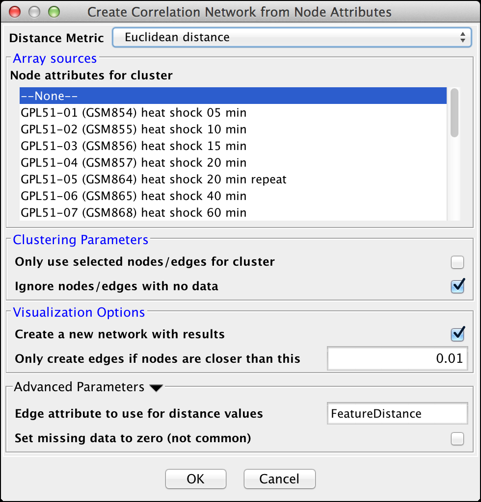
Figure 9. clusterMaker2 Create Correlation Network dialog.
- Distance Matrix:
- There are several ways to calculate the distance matrix that is used to
build the cluster. In clusterMaker2 these distances represent the
distances between two rows (usually representing nodes) in the matrix.
clusterMaker2 currently supports eight different metrics:
- Euclidean distance: this is the simple two-dimensional Euclidean distance between two rows calculated as the square root of the sum of the squares of the differences between the values.
- City-block distance: the sum of the absolute value of the differences between the values in the two rows.
- Pearson correlation: the Pearson product-moment coefficient of the values in the two rows being compared. This value is calculated by dividing the covariance of the two rows by the product of their standard deviations.
- Pearson correlation, absolute value: similar to the value above, but using the absolute value of the covariance of the two rows.
- Uncentered correlation: the standard Pearson correlation includes terms to center the sum of squares around zero. This metric makes no attempt to center the sum of squares.
- Uncentered correlation, absolute value: similar to the value above, but using the absolute value of the covariance of the two rows.
- Spearman's rank correlation: Spearman's rank correlation (ρ) is a non-parametric measure of the correlation between the two rows. This metric is useful in that it makes no assumptions about the frequency distribution of the values in the rows, but it is relatively expensive (i.e., time-consuming) to calculate.
- Kendall's tau: Kendall tau rank correlation coefficient (τ) between the two rows. As with Spearman's rank correlation, this metric is non-parametric and computationally much more expensive than the parametric statistics.
- None -- attributes are correlations: No distance calculations are performed. This assumes that the attributes are already correlations (probably only useful for edge attributes). Note that the attributes are also not normalized, so the correlations must be between 0 and 1.
Array sources
- Node attributes for cluster:
- This area contains the list of all numeric node attributes that can be used for calculating the distances between the nodes. One or more node attributes must be selected to perform the clustering.
Clustering Parameters
- Only use selected nodes/edges for cluster:
- Under certain circumstances, it may be desirable to cluster only a subset of the nodes in the network. Checking this box limits all of the clustering calculations and results to the currently selected nodes or edges.
- Ignore nodes/edges with no data:
- A common use of clusterMaker2 is to map data onto a pathway or protein-protein interaction network. Often the external data will not cover all of the nodes in the network, so the resulting clustering will have a number of "holes" that might make interpretation more difficult. If this box is checked, only nodes that have values for at least one of the attributes will be included in the matrix.
Visualization Options
- Create a new network
- If this option is selected, then a new network will be created with all of the nodes and the edges which represent the correlation between the nodes. An edge will only be created if the nodes are closer than the value specified in the next option. If this option is not selected, an attribute will be added to existing edges with the value of the correlation.
- Only create edges if nodes are closer than this:
- This value indicates the maximum correlation to consider when determining whether to create an edge or not. The correlation values are all normalized to lie between 0 and 1.
Advanced Parameters
- Edge attribute to use for distance values
- This is the name of the attribute to use for the distance values.
- Set missing data to zero (not common)
- In some circumstances (e.g. hierarchical clustering of edges) it is desirable to set all missing edges to zero rather than leave them as missing. This is not a common requirement.
3.3 Hierarchical Clustering
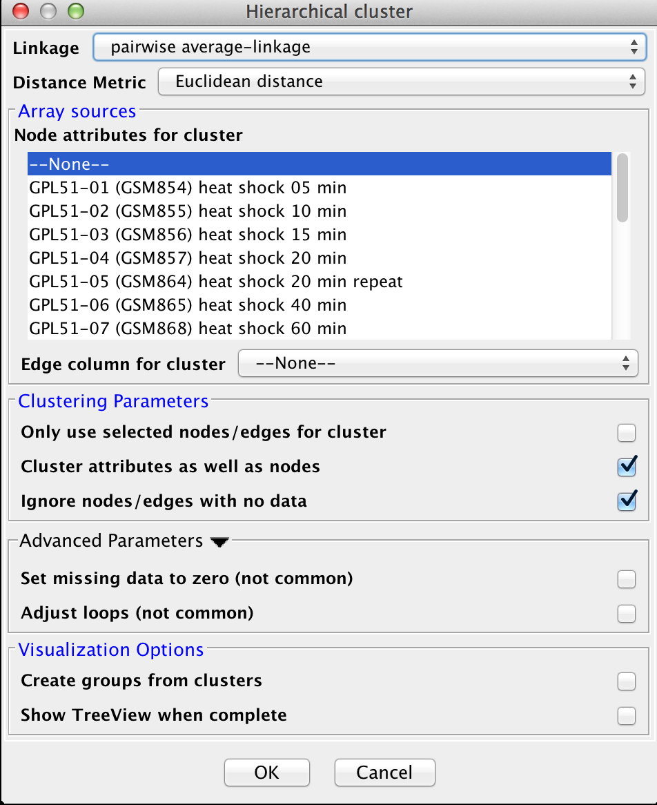
Figure 10. clusterMaker2 Hierarchical cluster dialog.
- Linkage:
- In agglomerative clustering techniques such as hierarchical clustering,
at each step in the algorithm, the two closest groups are chosen to be merged.
In hierarchical clustering, this is how the dendrogram (tree) is constructed.
The measure of "closeness" is called the linkage between the two groups.
Four linkage types are available:
- pairwise average-linkage: the mean distance between all pairs of elements in the two groups
- pairwise single-linkage: the smallest distance between all pairs of elements in the two groups
- pairwise maximum-linkage: the largest distance between all pairs of elements in the two groups
- pairwise centroid-linkage: the distance between the centroids of all pairs of elements in the two groups
- Distance Metric:
- There are several ways to calculate the distance matrix that is used to
build the cluster. In clusterMaker2 these distances represent the
distances between two rows (usually representing nodes) in the matrix.
clusterMaker2 currently supports eight different metrics:
- Euclidean distance: this is the simple two-dimensional Euclidean distance between two rows calculated as the square root of the sum of the squares of the differences between the values.
- City-block distance: the sum of the absolute value of the differences between the values in the two rows.
- Pearson correlation: the Pearson product-moment coefficient of the values in the two rows being compared. This value is calculated by dividing the covariance of the two rows by the product of their standard deviations.
- Pearson correlation, absolute value: similar to the value above, but using the absolute value of the covariance of the two rows.
- Uncentered correlation: the standard Pearson correlation includes terms to center the sum of squares around zero. This metric makes no attempt to center the sum of squares.
- Uncentered correlation, absolute value: similar to the value above, but using the absolute value of the covariance of the two rows.
- Spearman's rank correlation: Spearman's rank correlation (ρ) is a non-parametric measure of the correlation between the two rows. This metric is useful in that it makes no assumptions about the frequency distribution of the values in the rows, but it is relatively expensive (i.e., time-consuming) to calculate.
- Kendall's tau: Kendall tau rank correlation coefficient (τ) between the two rows. As with Spearman's rank correlation, this metric is non-parametric and computationally much more expensive than the parametric statistics.
- None -- attributes are correlations: No distance calculations are performed. This assumes that the attributes are already correlations (probably only useful for edge attributes). Note that the attributes are also not normalized, so the correlations must be between 0 and 1.
Array sources
- Node attributes for cluster:
- This area contains the list of all numeric node columns that can be used for calculating the distances between the nodes. One or more node attributes must be selected to perform the clustering.
- Edge column for cluster:
- An alternative to using multiple node columns for the clustering is to select a single edge column. In this case, the resulting clustering will be across the diagonal.
Clustering Parameters
- Only use selected nodes/edges for cluster:
- Under certain circumstances, it may be desirable to cluster only a subset of the nodes in the network. Checking this box limits all of the clustering calculations and results to the currently selected nodes or edges.
- Cluster attributes as well as nodes:
- If this box is checked, the clustering algorithm will be run twice, first with the rows in the matrix representing the nodes and the columns representing the attributes. The resulting dendrogram provides a hierarchical clustering of the nodes given the values of the attributes. In the second pass, the matrix is transposed and the rows represent the attribute values. This provides a dendrogram clustering the attributes. Both the node-based and the attribute-base dendrograms can be viewed, although Cytoscape groups are only formed for the node-based clusters.
- Ignore nodes/edges with no data:
- A common use of clusterMaker2 is to map expression data onto a pathway or protein-protein interaction network. Often the expression data will not cover all of the nodes in the network, so the resulting dendrogram will have a number of "holes" that might make interpretation more difficult. If this box is checked, only nodes (or edges, if using an edge column) that have values in at least one of the columns will be included in the matrix.
Advanced Parameters
- Set missing data to zero:
- In some circumstances (e.g. hierarchical clustering of edges) it is desirable to set all missing edges to zero rather than leave them as missing. This is not a common requirement.
- Adjust loops
- In some circumstances (e.g. hierarchical clustering of edges) it's useful to set the value of the edge between and node and itself to a large value. This is not a common requirement.
Visualization Options
- Create groups from clusters:
- If this button is checked, hierarchical Cytoscape groups will be created from the clusters. Hierarchical groups can be very useful for exploring the clustering in the context of the network. However, if you intend to perform multiple runs to try different parameters, be aware that repeatedly removing and recreating the groups can be very slow.
- Show TreeView when complete:
- If this option is selected, a JTree TreeView is displayed after the clustering is complete.
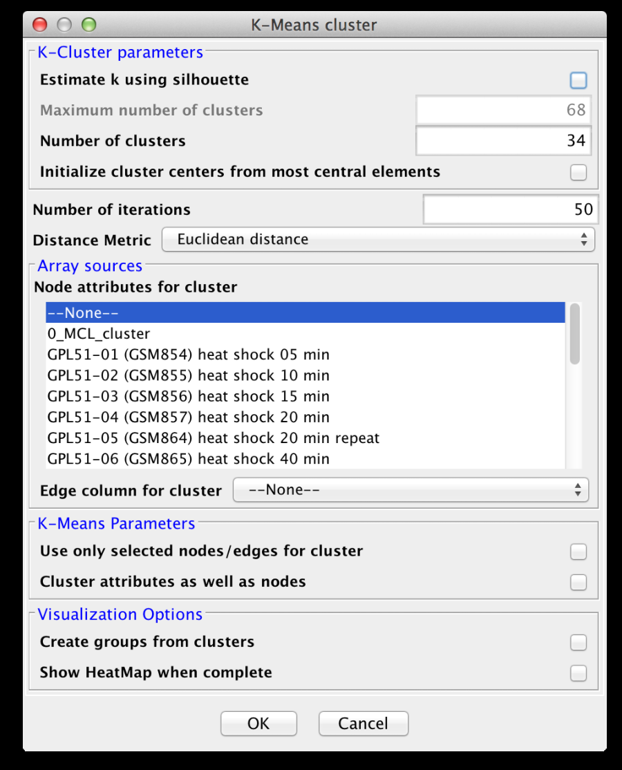
Figure 11. clusterMaker2 K-Means cluster dialog.
3.4 K-Means Clustering
K-Means clustering is a partitioning algorithm that divides the data into k non-overlapping clusters, where k is an input parameter. One of the challenges in k-Means clustering is that the number of clusters must be chosen in advance. A simple rule of thumb for choosing the number of clusters is to take the square root of ½ of the number of nodes. Beginning with clusterMaker2 version 1.6, this value is provided as the default value for the number of clusters. Beginning with clusterMaker2 version 1.10, k may be estimated by iterating over number of estimates for k and choosing the value that maximizes the silhouette for the cluster result. Since this is an iterative approach, for larger clusters, it can take a very long time, even though the process is multi-threaded. The K-Means cluster algorithm has several settings:K-Cluster parameters
- Estimate k using silhouette
- If this is checked, clusterMaker2 will perform k-means iteratively trying different values for k. It will then choose the value of k that maximizes the average silhouette over all clusters.
- Maximum number of clusters
- This is the maximum value for k that will be attempted when using silhouette to choose k.
- Number of clusters (k)
- This is the value clusterMaker2 will use for k if silhouette is not being used.
- Initialize cluster centers from most central elements
- If this is selected, the approach for cluster initialization is changed to use most central elements as opposed to random initialization.
- Number of iterations
- The number of iterations in the k-means algorithm.
- Distance Metric
- Array sources
K-Means Parameters
Visualization Options
- Create groups from clusters:
- If this button is checked, Cytoscape groups will be created from the clusters. Groups can be very useful for exploring the clustering in the context of the network. However, if you intend to perform multiple runs to try different parameters, be aware that repeatedly removing and recreating the groups can be very slow.
- Show HeatMap when complete:
- If this option is selected, a JTree KnnView is displayed after the clustering is complete.
3.5 K-Medoid Clustering
K-Medoid clustering is essentially the same as K-Means clustering except that the medoid of the cluster is used rather than the means to determine the goodness of fit. All other options are the same.3.6 HOPACH Clustering
HOPACH (Hierarchical Ordered Partitioning and Collapsing Hybrid) is a clustering algorithm that builds a hierarchical tree by recursively partitioning a data set with PAM -- sort of like an upside-down hierarchical cluster, but with a twist. At each level of the tree clusters are ordered and potentially collapsed. The Mean/Median Split Silhouette (MSS) criteria is used to identify the level of the tree with maximally homogeneous clusters.Basic HOPACH Tuning Parameters
- Distance Metric
- Split cost type:
- This setting determines the method used to determine the cost of splitting a cluster. The options are:
- Average split silhouette:
- Calculate the average split silhouette for the clusters
- Average silhouette:
- Calculate the average silhouette for the clusters
- Value summary method:
- This setting determines the method used to calculate the summary of the values for evalutating the cluster. It can either be Mean or Median.
- Maximum number of levels:
- The maximum number of levels in the tree. This value should be less than 16 for performance reasons.
- Maximum number of clusters at each level:
- A value between 1 and 9 secifying the maximum number of children at each node in the tree.
- Maximum number of subclusters at each level:
- A value between 1 and 9 secifying the maximum number of children at each node in the tree when calculating MSS. This is typically the same as the value above.
- Force splitting at initial level:
- If true, force the initial cluster to be split.
- Minimum cost reduction for collapse:
- A number between 0 and 1 speciying the margin of improvement in MSS to accept a collapse step.
Array Sources
HOPACH Parameters
Visualization Options
- Create groups from clusters:
- If this button is checked, Cytoscape groups will be created from the clusters. Groups can be very useful for exploring the clustering in the context of the network. However, if you intend to perform multiple runs to try different parameters, be aware that repeatedly removing and recreating the groups can be very slow.
- Show HeatMap when complete:
- If this option is selected, a JTree KnnView is displayed after the clustering is complete.
3.7 Partition Around Medoids (PAM) Clustering
PAM is a common clustering algorithm similar to k-Means and k-Medoid that uses a greedy search to partition the network.K-Cluster parameters
PAM Parameters
Visualization Options
- Create groups from clusters:
- If this button is checked, Cytoscape groups will be created from the clusters. Groups can be very useful for exploring the clustering in the context of the network. However, if you intend to perform multiple runs to try different parameters, be aware that repeatedly removing and recreating the groups can be very slow.
- Show HeatMap when complete:
- If this option is selected, a JTree KnnView is displayed after the clustering is complete.
4. Network Cluster Algorithms
The primary function of the network cluster algorithms is to detect natural groupings of nodes within the network. These groups are generally defined by a numeric edge attribute that contains some similarity or distance metric between two nodes, although some algorithms function purely on the existance of an edge (i.e. the connectivity). Nodes that are more similar (or closer together) are more likely to be grouped together.
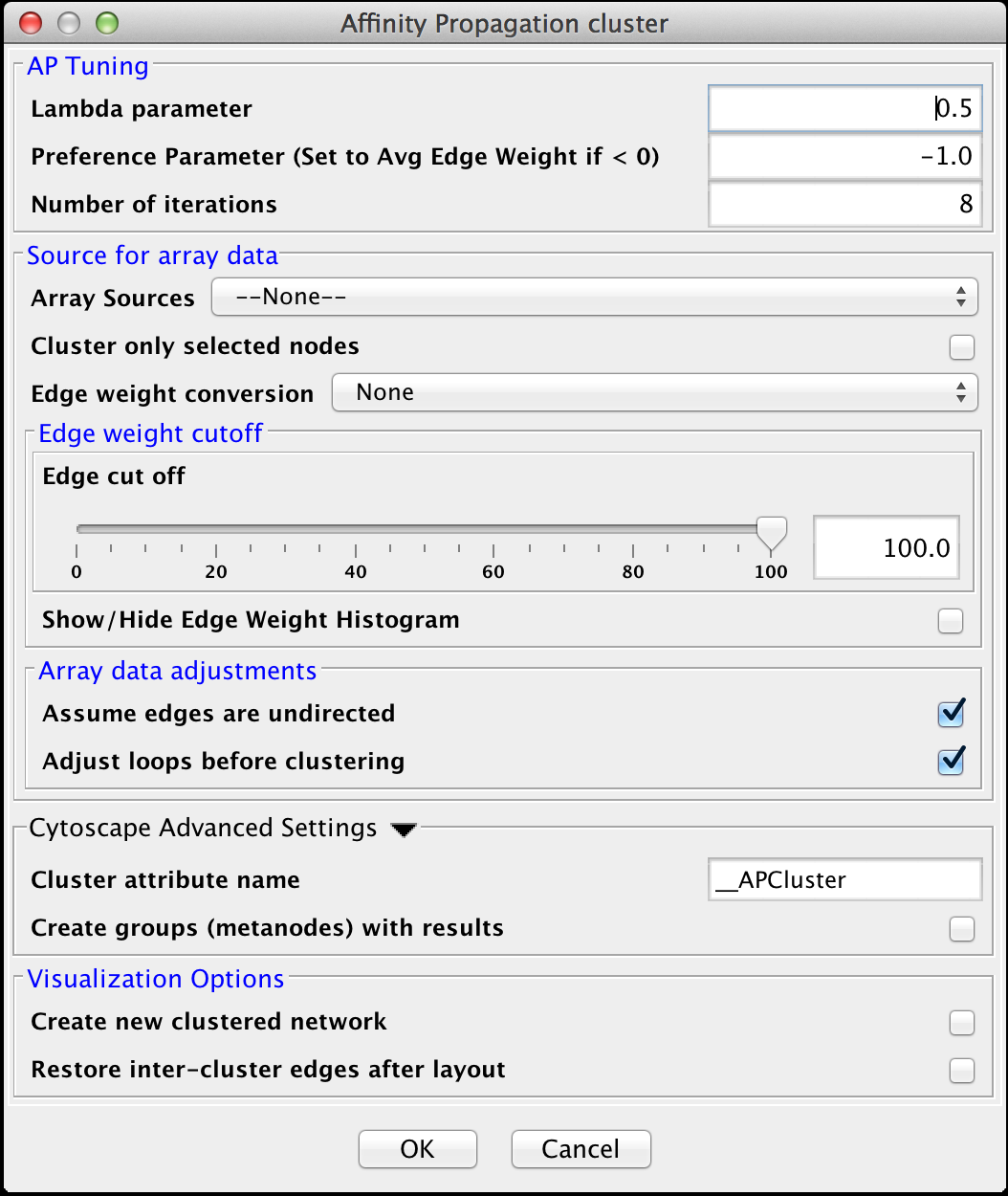
Figure 12. clusterMaker2 Affinity Propagation cluster dialog.
4.1 Affinity Propagation
Affinity Progation models the flow of data between points in a network in order to determine which of the points serve as data centers. These data centers are referred to as exemplars.Initally, AP considers all data points as potential exemplars. Real-valued messages are exhanged between data points at each iteration. The strength of the transmited messages determine the extent to which any given point serves as an exemplar to any other point. The quality of possible exemplar assignment is determined by a squared error energy function. Eventually, the algorithm reaches a minimal energy based on a good set of exemplars. The exemplars are then used to ouput the corresonding clusters. AP takes as input three parameters, which are discussed below.
AP Tuning
- Lambda Parameter:
- This parameter dampens the strengh of the message exchange at each iteration. Damping is necessary to avoid numerical oscillations that arise in some circumstances. Lambda may from 0 to .1. The default damping faction .5 tends to give adequate results.
- Preference Parameter:
- This parameter determines cluster density. It is analogous to the inflation parameter in MCL. Larger values for the preference parameter yield more clusters. If specified as less then zero, the preference value is automatically reset to the average edge weight in the network
- Number of iterations:
- Number of iterations the message exchange is run. 10 is usually enough to yield a stable set of exemplars
Source for array data
- Array sources:
- This pulldown contains all of the numeric edge attributes that can be used for this cluster algorithm. If is selected, all edges are assumed to have a weight of 1.0.
- Cluster only selected nodes:
- If this checkbox is selected, only the nodes (and their edges) which are selected in the current network are considered for clustering. This can be very useful to apply a second clustering to a cluster using a different algorithm or different tuning values.
- Edge weight conversion:
- There are a number of conversions that might be applied to the edge weights before clustering:
- None: Don't do any conversion
- 1/value: Use the inverse of the value. This is useful if the value is a distance (difference) rather than a similarity metric.
- LOG(value): Take the log of the value.
- -LOG(value): Take the negative log of the value. Use this if your edge attribute is an expectation value.
- SCPS: The paper describing the SCPS (Spectral Clustering of Protein Sequences) algorithm uses a special weighting for the BLAST expectation values. This edge weight conversion implements that weighting.
Edge weight cutoff
- Edge cut off
- Some clustering algorithms (e.g. MCL) have problems clustering very dense networks, even though many of the edge weights are very small. This value allows the user to set a custoff, either by directly entering a value, or using a slider to adjust the parameter. To view the histogram of edge weights (and set the edge weight cutoff on the histogram) use the Show/Hide Edge Weight Histogram checkbox.
- Show/Hide Edge Weight Histogram
- This checkbox acts like a toggle to show or hide the edge weight histogram dialog(see Figure 13).
The edge weight histogram dialog provides an interface to allow users to explore the histogram of edge
weights and interactively set the edge weights by dragging a slider along the histogram. The dialog supports five
buttons:
- Set Cutoff This puts a vertical line on the graph and allows the user to drag the line along to set the cutoff value. You must click into the historgram after pressing the button to activate the verticle line. The value and number of edges with that value are displayed at the top of the line (See Figure 13). The slider sets the value as it is dragged, so no further action is necessary once the desired cutoff is selected.
- Close Close the dialog.
- Zoom In Zooms in to the dialog (multiplies the width by 2). The histogram is placed in a scroll window so that the user may continue to have access to the entire histogram. This button may be pressed repeatedly.
- Zoom Out If the user has expanded the dialog with the Zoom In button, this button allows the user to zoom back out.
- Select Cutoff Heuristically This will calculate a candidate cutoff using the heuristic proposed by Apeltsin, et. al. (2011).
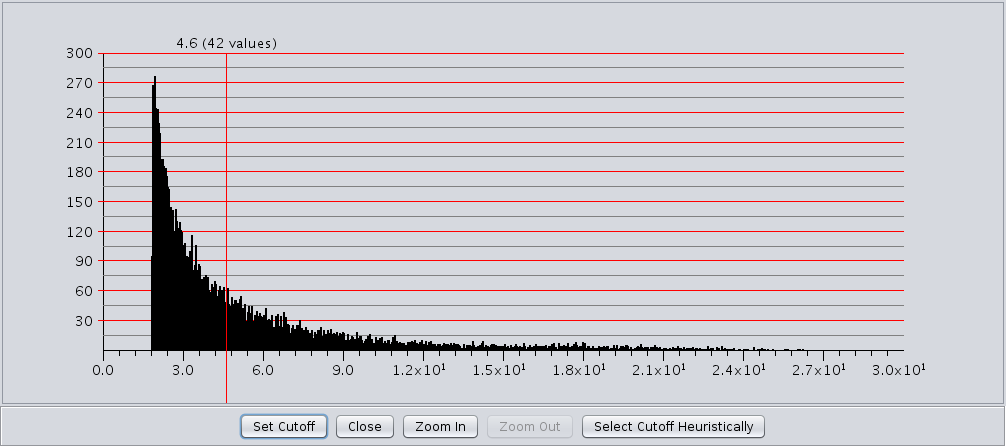
Figure 13. clusterMaker2 Edge Weight Histogram dialog with the Set Cutoff slider enabled.
Array data adjustments
- Assume edges are undirected:
- Some clustering algorithms take the edge direction into account, althrough most do not. Assuming the edges are undirected is normal. Not all algorithms support this value.
- Adjust loops before clustering:
- Loops refere to edges between a node and itself. Most networks do not include these as they cluster the visualization and don't seem informative. However, mathematically when the network is converted to a matrix these values become important. Checking this box sets these self-edges to the largest value of any edge in the row. Not all algorithms support this value.
Cytoscape Advanced Settings
- Cluster Attribute:
- Set the node attribute used to record the cluster number for this node. Changing this values allows multiple clustering runs using the same algorithm to record multiple clustering assignments.
- Create metanodes with results:
- Selecting this value directs the algorithm to create a Cytoscape metanode for each cluster. This allows the user to collapse and expand the clusters within the context of the network.
Visualization Options
- Create new clustered network
- If this option is selected, after the clustering is complete, a new network will be generated with the edges between clusters removed. A view for the resulting network will be created and laid out using the Force Directed layout.
- Restore inter-cluster edges after layout
- If this option is selected, after the clustered network is created and laid out, the edges that were removed are added back in. See Figure 12 for an example.
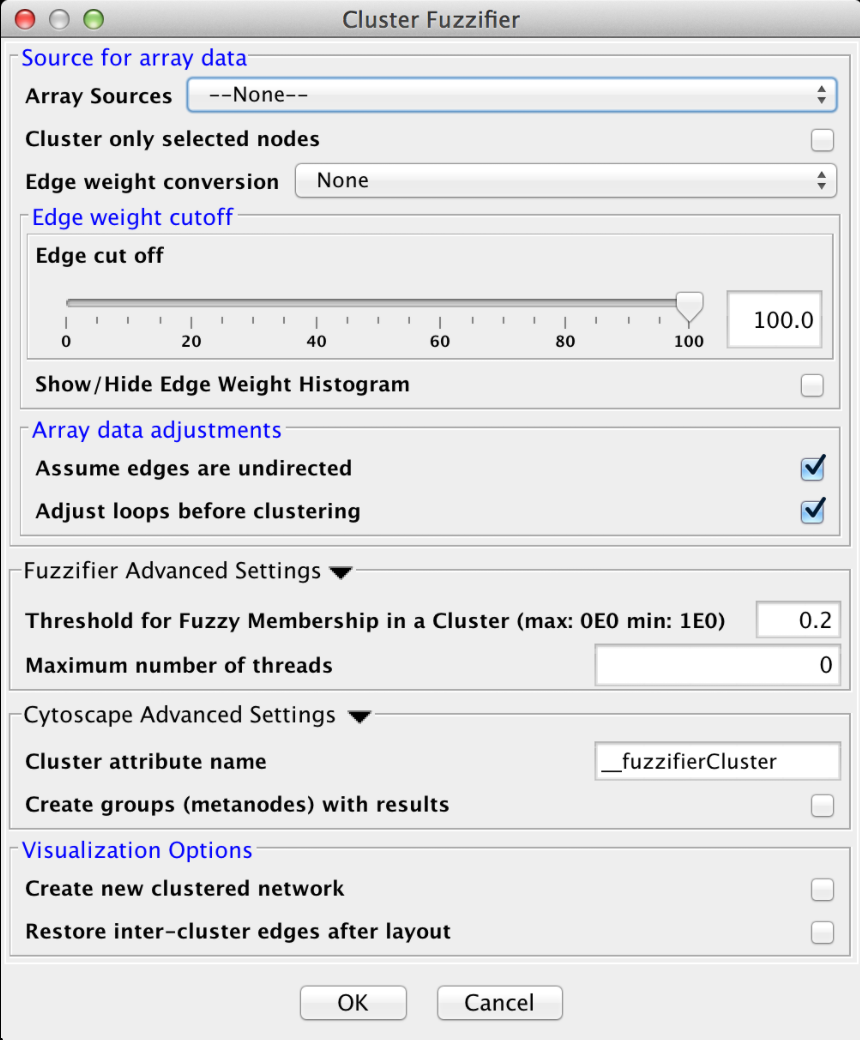
Figure 14. clusterMaker2 Cluster Fuzzifier dialog.
4.2 Cluster "Fuzzifier"
In biology, partitions are rarely "hard", and most biological measures involve some degree of "fuzzyness". On the other hand, most of the network clustering algorithms developed for biology do hard partitioning. For example, partioning a protein-protein interaction network to determine stable complexes, or partioning a protein-protein similarity network to annotate proteins into functional groups. In both of these cases, the actual biology gives a more nuanced view than the clustering algorithm provides. For example, proteins that are members of multiple complexes will be assigned to only one in hard clustering. This algorithm is an initial step to restore some of the missing nuance lost in a hard clustering without reinventing the clustering algorithm itself. It takes a very simple approach of fuzzifying an existing cluster result (that is restoring partial membership information to the existing hard partitioning). It does this by calculating the centroid of each cluster, similar to fuzzy c-means (see below) and determining the distance of a node from that centroid. This membership information may be visualized as additional membership edges in the network.
Array Sources
Edge weight cutoff
Array data adjustments
Fuzzifier Advanced Settings
- Threshold for Fuzzy Membership in a cluster
- This is the minimum value for a node to be considered part of a cluster measured as a proportion of membership. For example, a node that is halfway inbetween two clusters might have a proportional membership of .5 in each. Nodes that are outside of this threshold are not included in the resulting network.
- Maximum number of threads
- The maximum number of threads to use for the estimate for the number of clusters. The actual number of threads used will depend on the number of processors available on the machine.
Cytoscape Advanced Settings
Visualization Options

Figure 15. clusterMaker2 Community cluster (GLay) dialog.
4.3 Community Clustering (GLay)
The community clustering algorithm is an implementation of the Girvan-Newman fast greedy algorithm as implemented by the GLay Cytoscape plugin. This algorithm operates exclusively on connectivity, so there are no options to select an array source, although options are provided to Cluster only selected nodes and Assume edges are undirected. It supports all of the Cytoscape Advanced Settings options, as well as the Visualization Options.
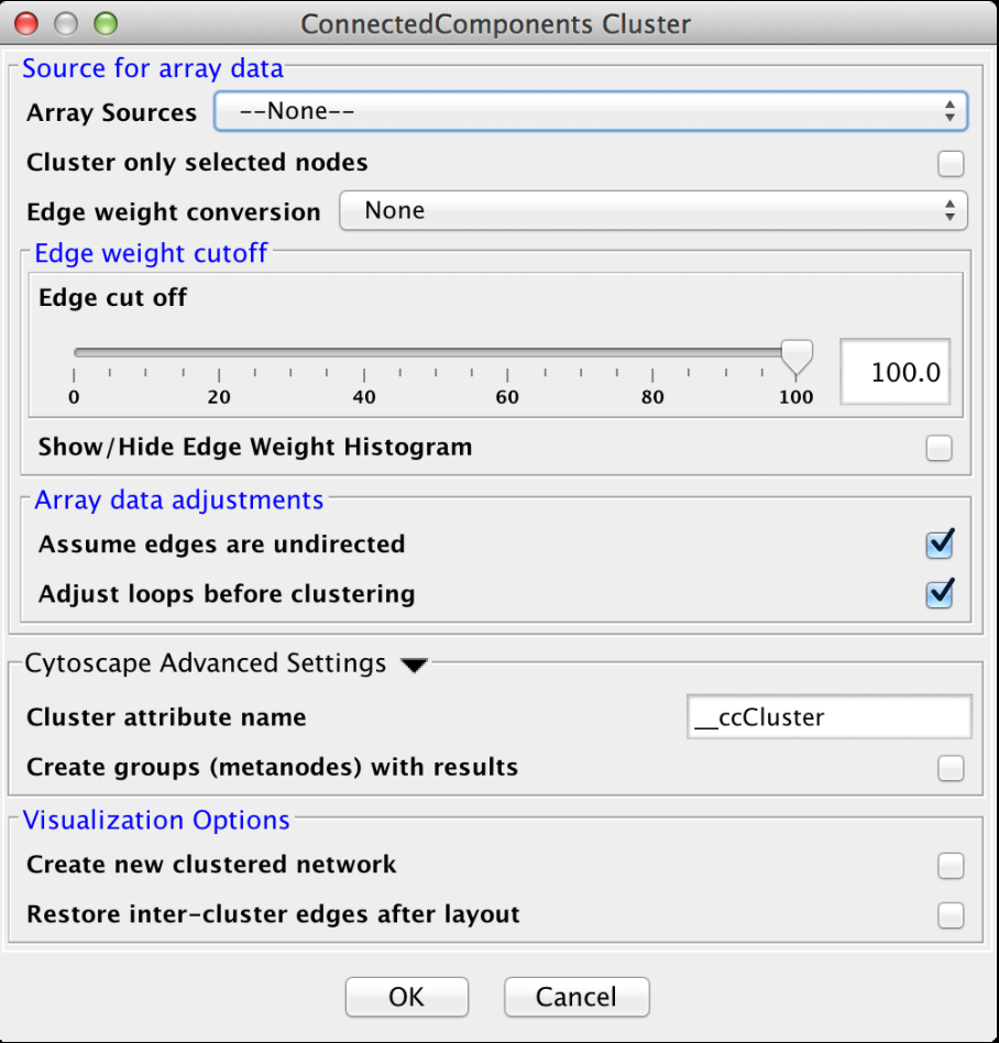
Figure 16. clusterMaker2 Connected Components cluster dialog.
4.4 Connected Components
This is a very simple "cluster" that simply finds all of the disconnected components of the network and treats each disconnected component as a cluster. It supports the Array Sources, Array Data Adjustments, Cytoscape Advanced Settings, and Visualzation Options options. Figure 16 shows the options panel for the Connected Components cluster.
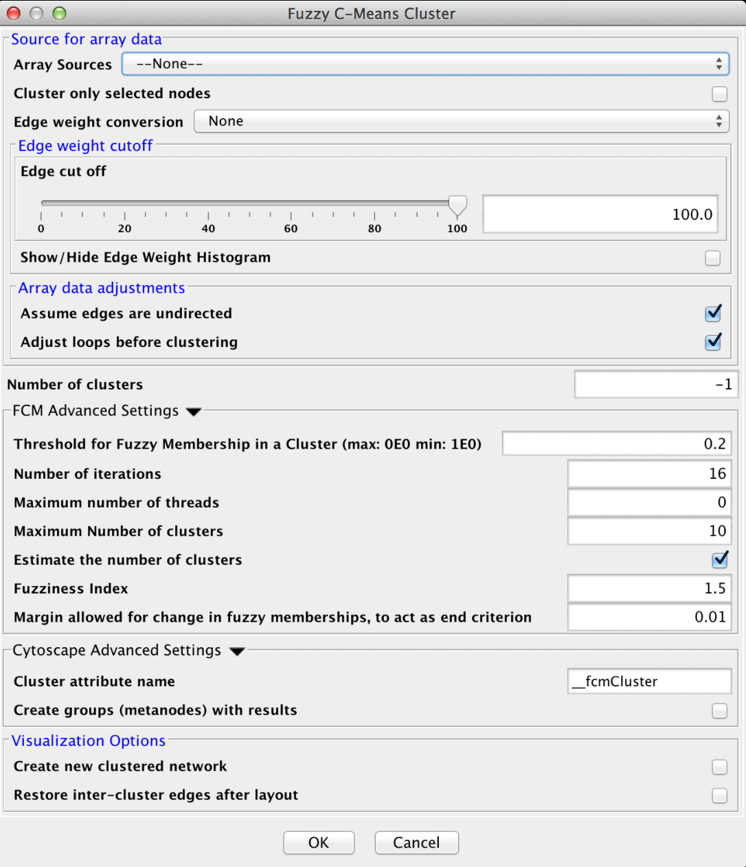
Figure 17. clusterMaker2 Fuzzy C-Means cluster dialog.
4.4 Fuzzy C-Means
Fuzzy C-Means is a fuzzy clustering algorithm that is similar to k-means. It is "fuzzy" in that a node may belong to more than one cluster. The algorithm calculates the "degree of membership" (or probability of membership" based on the distance between a node and the centroid of the cluster as calculated by taking the mean of all members. Like k-means, this algorithm assumes that the number of clusters is known (although in our implementation, it may be estimated).
Array Sources
Edge weight cutoff
Array data adjustments
- Number of clusters
- The number of clusters to create. If this value is -1 the number of clusters is estimated by finding the best k for values between 2 and Maximum Number of clusters, where the "goodness" of the cluster is measured using the silhouette measure.
FCM Advanced Settings
- Threshold for Fuzzy Membership in a Cluster
- This value indicates the minimum membership proportion necessary to consider a node a member of a cluster. The default value of 0.2 indicates that a node must be at least 20% a part of the cluster before we include it in the list of members
- Number of iterations
- The maximum number of iterations of the algorithm before taking the result. If the algorithm converges (no more changes in fuzzy membership) then it will exit before this number of iterations, otherwise it will wait until all iterations have completed before existing.
- Maximum number of threads
- The maximum number of threads to use for the estimate for the number of clusters. The actual number of threads used will depend on the number of processors available on the machine.
- Maximum number of clusters
- When estimating the number of clusters, this is the upper bound to try.
- Estimate the number of clusters
- If checked, estimate the number of clusters by running all possible clusters between 2 and the maximum number of clusters and pick the number that gives the best silhouette value.
- Fuzziness Index
- This value indicates the amount of weight given to the closest center when calculating the degree of membership
- Margin allowed for change in fuzzy memberships
- This represents the end criteria for the algorithm. If the change in fuzzy memberships does not exceed this value, then the algorithm has converged and the clusters are returned.
Cytoscape Advanced Settings
Visualization Options
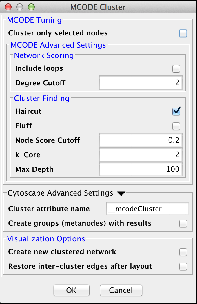
Figure 18. clusterMaker2 MCODE cluster dialog.
4.5 MCODE
The MCODE algorithm finds highly interconnected regions in a network. The algorithm uses a three-stage process:
- Vertex weighting, which weights all of the nodes based on their local network density.
- Molecular complex prediction, staring with the highest-weighted node, recursively move out adding nodes to the complex that are above a given threshold.
- Post-processing, which applies filters to improve the cluster quality.
MCODE Tuning
- Cluster only selected nodes:
- If this checkbox is selected, only the nodes (and their edges) which are selected in the current network are considered for clustering. This can be very useful to apply a second clustering to a cluster using a different algorithm or different tuning values.
Advanced Tuning Options
- Include loops:
- If checked, loops (self-edges) are included in the calculation for the vertex weighting. This shouldn't have much impact
- Degree Cutoff:
- This value controls the minimum degree necessary for a node to be scored. Nodes with less than this number of connections will be excluded.
- Haircut:
- If checked, drops all of nodes from a cluster if they only have a single connection to the cluster.
- Fluff:
- If checked, after haircutting (if checked) all of the cluster cores are expanded by one step and added to the cluster if the score is greater than the Node Score Cutoff.
- K-Core:
- Filters out clusters that do not conatin a maximally interconnected sub-cluster of at least k degrees.
- Max Depth:
- This controls how far out from the seed node the algorithm will search in the molecular complex prediction step.
Network Scoring
Cluster Finding
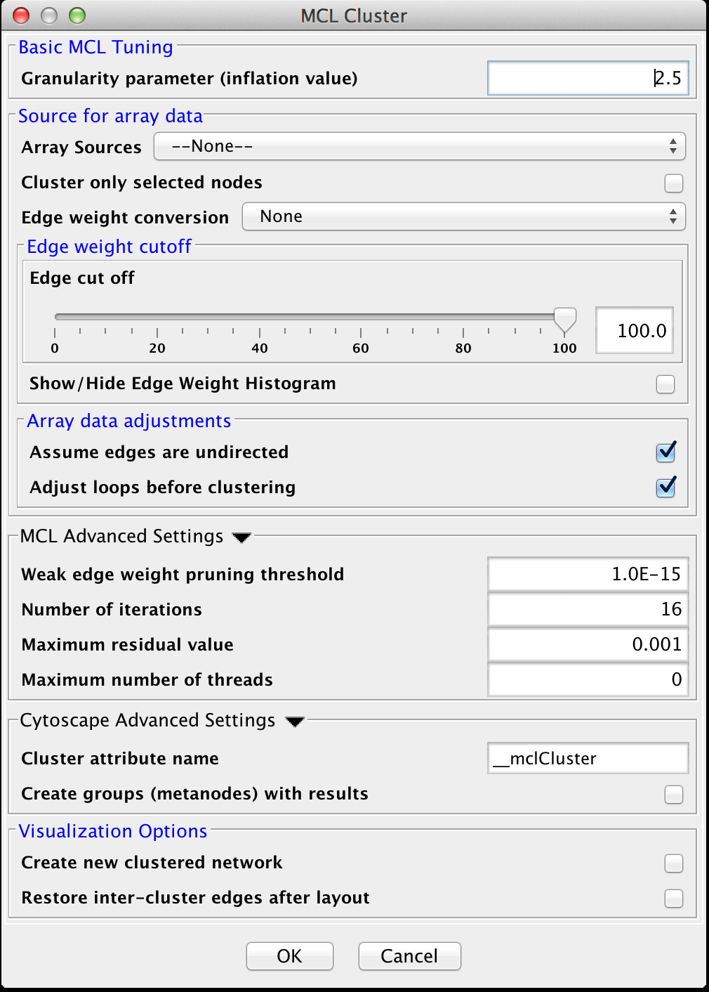
Figure 19. clusterMaker2 MCL cluster dialog.
4.6 MCL
Markov CLustering Algorithm (MCL) is a fast divisive clustering algorithm for graphs based on simulation of the flow in the graph. MCL has been applied to complex biological networks such as protein-protein similarity networks. As with all of the clustering algorithms, the first step is to create a matrix of the values to be clustered. For MCL, these values must be stored in edge attributes. Once the matrix is created, the MCL algorithm is applied for some number of iterations. There are two basic steps in each iteration of MCL. First is the expansion phase where the matrix is expanded by calculating the linear algebraic matrix-matrix multiplication of the original matrix times an empty matrix of the same size. The next step is the inflation phase where the each non-zero value in the matrix is raised to a power followed by performing a diagonal scaling of the result. Any values below a certain threshold are dropped from the matrix after the normalization (scaling) step in each iteration. This process models the spreading out of flow during expansion, allowing it to become more homogeneous, then contracting the flow during inflation, where it becomes thicker in regions of higher current and thinner in regions of lower current. This version of the MCL algorithm has been parallelized to improve performance on multicore processors.
The MCL dialog is shown in Figure 19. MCL has one parameter and supports the Array Sources and the Cytoscape Advanced Settings options, as well as a set of four advanced settings. Each parameter is discussed below:
Basic MCL Tuning
- Granularity Parameter (inflation value)
- The Granularity Parameter is also known as the inflation parameter or inflation value. This is the power used to inflate the matrix. Reasonable values range from ~1.8 to about 2.5. A good starting point for most networks is 2.0.
Source for array data
Edge weight cutoff
Array data adjustments
MCL Advanced Settings
- Weak Edge Weight Pruning Threshold
- After each inflation pass, very small edge weights are dropped out. This should be a very small number: 1x10⁻¹⁰ or so. The algorithm is more sensitive to tuning this parameter than it is to tuning the inflation parameter. Changes in this parameter also significantly impact the performance.
- Number of iterations
- This is the maximum number of iterations to execute the algorithm.
- The maximum residual value
- After each iteration, the residuals are calculated, and if they are less than this value, the algorithm is terminated. Set this value very small to ensure that you get sufficient iterations.
- The maximum number of threads
- If the machine has multiple cores or CPUs, MCL will by default utilize nCPUs-1 for it's operations. So, on an Intel i7 with 4 cores and hyperthreading, MCL will utilize 7 threads (4 cores X 2 hyperthreads) - 1 = 7. If this parameter is set to something other than 0, MCL will ignore the above calculation and utilize the specified number of threads.
Cytoscape Advanced Settings
Visualization Options
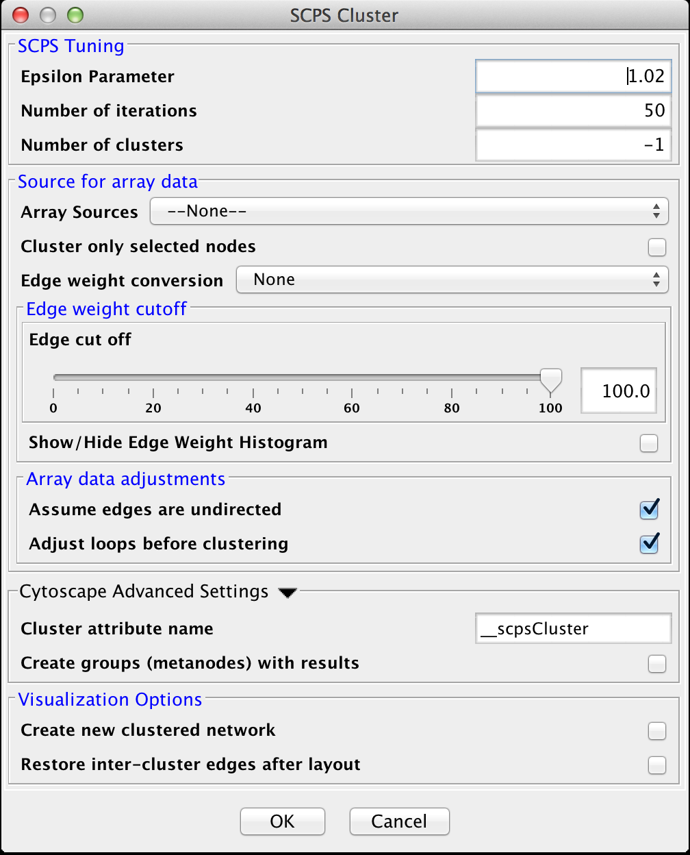
Figure 20. clusterMaker2 SCPS cluster dialog.
4.7 SCPS (Spectral Clustering of Protein Sequences)
SCPS is a spectral method designed for grouping proteins. Spectral methods use the eigenvalues in an input similarity matrix to perform dimensionality reduction for clustering in fewer dimensions. SCPS builds a matrix from the k largest eigenvectors, where k is the number of clusters to be determined. A normalized transpose of that matrix is then used as input into a standard k-means clustering algorithm. The user may specify the Number of clusters parameter with a preset value of k, as well as the Number of iterations that k-means is to be run. However, if the user does not know the value of k in advance, he or she may set the Number of clusters to -1, and SCPS will pick a value for k using an automated heuristic. The heuristic picks the smallest integer k such that the ratio of the kth eignevalue and the k+1st eigenvalue is greater then the Epsilon Paramter. An epsilon of 1.02 is good for clustering diverse proteins into superfamilies. A more granular epsilon of 1.1 may cluster proteins into functional families.
SCPS Tuning
- Epsilon Parameter:
- The epsilon parameter to use.
- Number of Iterations:
- The number of iterations for the k-means clustering.
- Number of clusters:
- The number of clusters. If this is -1, SCPS will pick a value for k using an automated heuristic.
Array Sources
Edge weight cutoff
Array data adjustments
Cytoscape Advanced Settings
Visualization Options
Figure 21. clusterMaker2 Transitivity cluster dialog.
4.8 Transitivity Clustering
TransClust is a clustering tool that incorporates the hidden transitive nature occuring within biomedical datasets. It is based on weighed transitive graph projection. A cost function for adding and removing edges is used to transform a network into a transitive graph with minimal costs for edge additions and removals. The final transitive graph is by definition composed of distinct cliques, which are equivalent to the clustering output.
Array Sources
Edge weight cutoff
Array data adjustments
Advanced Tuning Parameters
- Max. Subcluster Size:
- The maximum size of a subcluster. This option adjusts the size of subproblems to be saved exactly. The higher the number, the higher the running time but also the accuracy. For fast computers, you may want to set this value to 50.
- Max. Time (secs):
- The maximum time, in seconds, to execute each loop in the algorithm. Increasing this parameter raises both running time and accuracy. For fast computers, you may want to set this value to 2.
- Merge very similar nodes to one?:
- If this it true, nodes exceeding a threshold parameter will be merged be merged virtually into one object while clustering. This may decrease running time drastically.
- Threshold:
- The threshold for merging nodes the merge parameter is activated. For protein sequence clustering using BLAST as a smiliarity function, it might make sense to set the threshold at 323, since this is the highest reachable similarity.
- Number of Processors:
- The number of processors (threads) to use.
Find Exact Solution
Merge nodes
Parallel computing
Cytoscape Advanced Settings
Visualization Options
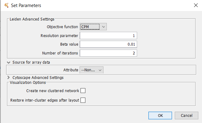
Figure 22. clusterMaker2 Leiden cluster dialog.
4.9 Leiden Clustering (remote)
The Leiden algorithm is an improvement of the Louvain algorithm. It consists of three phases: local moving of nodes, refinement of the partition aggregation of the network based on the refined partition, using the non-refined partition to create an initial partition for the aggregate network.Array Sources
Array data adjustments
Leiden Parameters
- Objective function
- Whether to use the Constant Potts Model (CPM) or modularity. Must be either "CPM" or "modularity".
- Resolution Parameter
- The resolution parameter to use. Higher resolutions lead to more smaller communities, while lower resolutions lead to fewer larger communities.
- Beta Value
- Parameter affecting the randomness in the Leiden algorithm. This affects only the refinement step of the algorithm.
- Number of iterations
- The number of iterations to iterate the Leiden algorithm. Each iteration may improve the partition further.
Visualization Options

Figure 23. clusterMaker2 Infomap dialog.
4.10 Infomap (remote)
Infomap is a network clustering algorithm based on the Map equation.Array Sources
Array data adjustments
Infomap Parameters
- Trials
- The number of attempts to partition the network.
Visualization Options
4.11 Fast Greedy (remote)
This function tries to find dense subgraph, also called communities in graphs via directly optimizing a modularity score.Array Sources
Array data adjustments
Fast Greedy Parameters
-
No adjustable parameters.
Visualization Options
4.12 Leading Eigenvector (remote)
These functions try to find densely connected subgraphs in a graph by calculating the leading non-negative eigenvector of the modularity matrix of the graph.Array Sources
Array data adjustments
Leading Eigenvector Parameters
-
No adjustable parameters.
Visualization Options
4.13 Label Propagation (remote)
The Label Propagation algorithm (LPA) is a fast algorithm for finding communities in a graph. It detects these communities using network structure alone as its guide, and doesn’t require a pre-defined objective function or prior information about the communities. LPA works by propagating labels throughout the network and forming communities based on this process of label propagation. The intuition behind the algorithm is that a single label can quickly become dominant in a densely connected group of nodes, but will have trouble crossing a sparsely connected region. Labels will get trapped inside a densely connected group of nodes, and those nodes that end up with the same label when the algorithms finish can be considered part of the same community.Array Sources
Array data adjustments
Label Propagation Parameters
-
No adjustable parameters.
Visualization Options
4.14 Multilevel Clustering (remote)
Multilevel Clustering measures similarity within a community of users using local and global information, modelling structural and intrinsic textual features jointly.Array Sources
Array data adjustments
Multilevel Parameters
-
No adjustable parameters.
Visualization Options
5. Filtering Clusters
Filters are a tool to "fine tune" clusters after a clustering algorithm has completed. In general, the idea behing the filters are to examine the results of a clustering algorithm and, based on some metric, trim the edges (drop nodes) or add edges to improve the clustering. The goal is to reduce noise and increase the cluster quality.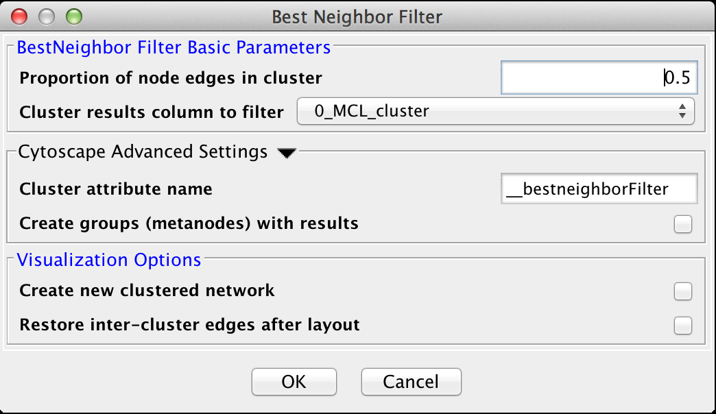
Figure 24. The settings dialog for the Best Neighbor Filter.
5.1 Best Neighbor Filter
The Best Neighbor filter is a filter which will add nodes and edges to a cluster when a neighboring node is a better fit in this cluster based on the number of edges from that node into this cluster.BestNeighbor Filter Basic Parameters
- Proportion of node edges in cluster
- The proportion of edges for this node that are a member of the cluster. Note that this is unweighted, so care should be exersized when using this filter
- Cluster results column to filter
- This is the attribute that contains the cluster numbers to use for the filtering.
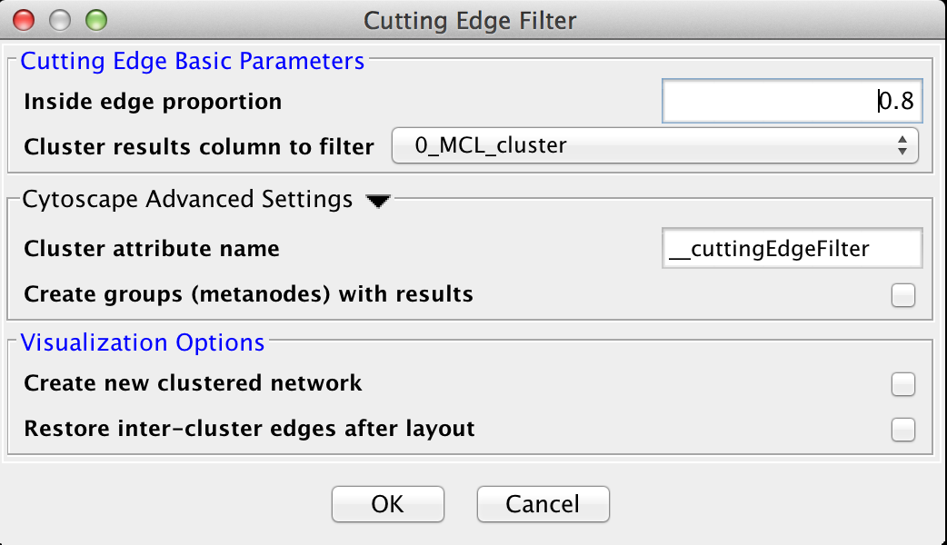
Figure 25. The settings dialog for the Cutting Edge Filter.
5.2 Cutting Edge Filter
Cutting Edge is a relatively coarse filter that discards clusters that don't meet the criteria. The criteria is defined as a density value where the cluster density is equal to the number of intra-cluster edges divided by the total number of edges (both intra-cluster and inter-cluster) that connect to nodes belonging to this cluster. If the density is less than the value, the cluster is dropped. The Cutting Edge Filter has the following values:Cutting Edge Basic Parameters
- Inside edge proportion
- The proportion of inside edges to total edges. Values can vary from 0 to 1 where 0 implies that the cluster has no inside edges and 1 implies that all of the edges are inside edges.
- Cluster results column to filter
- This is the attribute that contains the cluster numbers to use for the filtering.

Figure 26. The settings dialog for the Density Filter.
5.3 Density Filter
This filter drops clusters which have an edge density beneath the user-defined threshold. A fully connected network (all nodes are connected to all other nodes) will have an edge density of 1. A completely disconnected network will have an edge density of 0. The Density Filter has the following values:Density Filter Basic Parameters
- Minimum density
- The minimum density a cluster must have to be retained, where 0 implies that the cluster has no inside edges and 1 implies that all of the nodes are connected to all other nodes (fully connected).
- Cluster results column to filter
- This is the attribute that contains the cluster numbers to use for the filtering.
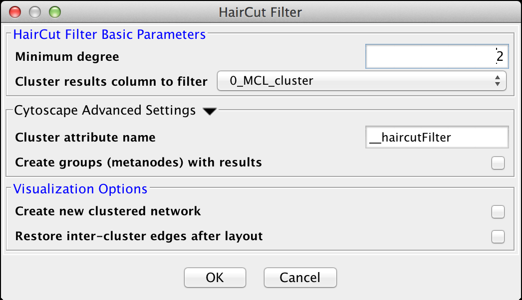
Figure 27. The settings dialog for the Haircut Filter.
5.4 Haircut Filter
The haircut filter removes nodes from a cluster that have a degree (number of incident edges) below a specified value. The idea is that the lower the connectivity of a node, the lower the probability for this node to really belong to the cluster it is in. The Haircut Filter has the following values:HairCut Filter Basic Parameters
- Minimum degree
- This is the minimum degree for a node to be kept within the cluster.
- Cluster results column to filter
- This is the attribute that contains the cluster numbers to use for the filtering.
6. Ranking Clusters
These algorithms were developed and added to clusterMaker2 by Henning Lund-Hanssen as part of his Master's work at the University of Oslo. For background on the motivation and details on the implementation, see his Thesis entitled: Ranklust: An extension of the Cytoscape clusterMaker2 plugin and its application to prioritize network biomarkers in prostate cancer, 2016. The general idea behind the inclusion of these algorithms into clusterMaker2 is the desire to attempt to rank the results of a clustering result based on potentially orthogonal information. For example, a user could use MCL clustering to partition a network based on an edge weight, then use node attribute information (e.g. expression data) to rank those clusters. In order to use any of the techniques below, the network should first be clustered using one of the network partitioning cluster algorithms (e.g. MCL) and a new network should be created without adding back the inter-cluster edges. Then select that network to use the following algorithms. The text below is taken from the above cited thesis. Results from cluster ranking may be displayed in the6.1 Multiple nodes and edges (Additive sum)
The multiple attribute additive (MMA) panel provides the user the option of choosing an unlimited amount of attributes from nodes and edges.
MMA goes through all of the nodes in each cluster and sums up the number- attributes the user chose. Each cluster is then ranked based on the average sum in each cluster and ranked descending, with the highest ranking cluster as the most likely prostate cancer biomarker cluster.
There is a question as to how to rank the edges in the cluster. We chose to rank each edge as it is listed to the user in Cytoscape. So if it is listed only once time in the edge table, it will only be scored additively once. This decision was based on simplicity. To not represent the edge as something the user did not define it as, or is unable to understand. Some clustering algorithms might assign the same node or edge to several clusters, though this is not the case with the algorithms I use in this thesis. Support for this is only implemented by MAA and MAM, as they were implemented before a final decision on which clustering algorithms should be used. If MAA/MAM discovers this special case of several scores for a single node or edge, it will assign it the highest value. The reason for leaving this feature in Ranklust is to have an example on how it can be done, should it be a problem in the future.
6.2 Multiple nodes and edges (Multiply sum)
Multiple attribute multiplication (MAM) method is to some degree redundant, considering what exists from before in clusterMaker2 cluster ranking. The only difference from MAA is the scale the scores will be in. MAA adds the scores from each node and edge in the cluster through addition, MAM does it with multiplication.
A problem that occurs with multiplication is calculating scores for clusters that contain nodes with a score between 0 and 1, since the score would decrease to such a degree that it would be difficult to work with when normalizing the scores. The solution I have chosen for this problem is to make a new score from the score that is to be added to the cluster average, and add 1.0 to it. This way, when the existing average score in the cluster is multiplied with the new score, it will always increase, unless the old value was 0.0, or both the old and the new value was 1.0. In the case of values above 1, they will also be given an increase by 1.0 in order to keep it consistent if the scores vary between 0 to n. Normalizing every value before running the algorithm contributes to keep all of the values between 0 and 1, and in that way prevent scaling problems when adding 1.0 to a score over 1.0. The whole reason to add 1.0 was to counteract the problem with the score decreasing when it should be increasing.
6.3 PageRank
Discussed below as part of PRWP.6.4 PageRank with Priors
A Random Walks algorithm which used priors, called seed-weighted random walks ranking, proved to be effective at prioritizing biomarker candidates. PageRank (PR) is an algorithm based on the Random Walks principle, and was previously used by Google to rank webpages. PageRank with Priors (PRWP) is a modified version of PR, where nodes and edges can be assigned a score prior to the PR’s traversal of the network. PR can have values assigned to the edges, but it does not require any scores in order to rank clusters, which PRWP does.
The difference between MAA and MAM compared to PR and PRWP is how the network is scored. MAA and MAM calculates the score for each cluster by summing up the attributes in edges and nodes according to the cluster attribute. PRWP scores the current network regardless of the clustering attribute.
MCL gives the option of creating a clustered network, which opens up the possibility of working with two types of the same network, non-clustered and clustered. They both have the clustering attribute in the network, edge and node table, so that the ranking algorithms are able to score the clusters. PRWP scores the currently selected network in Cytoscape, resulting in the option of scoring the non-clustered network or clustered network. The last option gives the clustering algorithm a bigger impact on the score, because the clustered network has perturbated edges between nodes that is not in the same cluster. MCL in Cytoscape can show the "inter-cluster" connecting edges, which is the egdes that was perturbed during clustering. This last option is a combination of the two others. It will be visually close to the clustered network, but algorithms that run on the network with inter- cluster edges will have the same result as the network only containing the cluster attribute.
Implementation wise, there is also a difference in how the scores are stored in the network after the algorithm is finished executing. All the scores are stored in the nodes. To give information to the user about the scores the edges received, each edge will display the total score for the cluster it is a member of, just like the nodes. Only PRWP and PR will also display the single node score.
6.5 Hyperlink Induced Topic Search
Hyperlink-Induced Topic Search, HITS, an algorithm that is similar to PageRank, was developed around the same time. HITS will not be used to calculate cluster scores and ranks, due to the fact that it does not require any form of weighting in nodes or edges. Though, it can be used in combination with other ranking algorithms through the use of MAM or MAA.An example of this could be running PRWP with a score attribute, then HITS on the same network. The next step would be to combine the two scores from PRWP and HITS with MAA.
7. Dimensionality Reduction
New in clusterMaker2 version 1.1 and later is the addition of algorithms for performing dimensionality reduction. A reasonable discussion of dimensionality reduction analysis is available in Wikipedia.
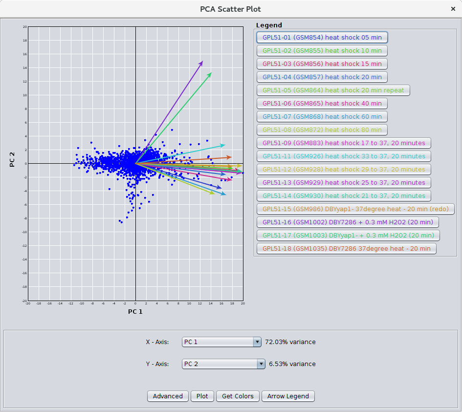
Figure 28. The PCA Scatter Plot.
7.1 Principal Components Analysis
The main linear technique for dimensionality reduction, principal component analysis, performs a linear mapping of the data to a lower-dimensional space in such a way that the variance of the data in the low-dimensional representation is maximized. In practice, the covariance (and sometimes the correlation) matrix of the data is constructed and the eigen vectors on this matrix are computed. The eigen vectors that correspond to the largest eigenvalues (the principal components) can now be used to reconstruct a large fraction of the variance of the original data. The clusterMaker2 implementation of PCA provides the ability to choose covariance or correlation.
Array Sources
- Node attributes for PCA:
- Choose the list of attributes to use for the analysis
- Only use selected nodes for PCA:
- Restricts the calculation to a subset of the network
- Ignore nodes with no data:
- If none of the attributes has a value for a node, that node is excluded
PCA Parameters
- Type of matrix to use for PCA:
- The type of matrix to use for the principal components:
- covariance:
- Compute the covariance matrix
- correlation:
- Compute the correlation matrix
- Standardize data?:
- If this is checked, the input data is standardized by adjusting each column by subtracting the mean of the column from each data item and dividing by the standard deviation.
Result Options
- Create PCA Result Panel:
- Adds a new tab to the results panel with each principal component. Selecting the component will select all of the nodes in the network that are part of that component
- Create PCA scatter plot:
- If checked, after the PCA calculation is complete, a scatter plot is displayed (see Figure 28). The scatter plot includes the loading vectors for each node attribute as well as options to color the loading vectors, select the components to use for the X and Y axes.
- Minimum variance for components (%):
- This sets the minimum explained variance for a component to be considered for display in the scatter plot.
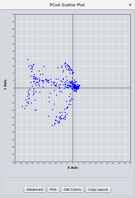
Figure 29. The PCoA Scatter Plot.
7.2 Principal Coordinates Analysis
Principal coordinates analysis (PCoA; also known as metric multidimensional scaling) summarises and attempts to represent inter-object (dis)similarity in a low-dimensional, Euclidean space. PCoA is similar to PCA except that it takes a dissimilarity matrix rather than a matrix, which makes it better suited to performing dimensionality reduction on the variance in edge attributes. Note that you must make sure that you convert your edge attribute values to distances (e.g. smaller is better) rather than weights (larger is better).Source for Array Data
Edge weight cutoff
Array data adjustments
PCoA Parameters
- Negative eigenvalue handling:
- Changes how the algorithm deals with negative eigenvalues:
- Discard:
- The default -- just discard the values
- Keep:
- Keep the negative eigenvalues
- Correct:
- Attempt to correct the negative eigenvalues
Result Options
- Create PCoA scatter plot:
- If checked, after the PCoA calculation is complete, a scatter plot is displayed (see Figure 29). The scatter plot only includes the first 2 components, organized as X and Y. Buttons allow the user to map node colors from the network view to the scatter plot and to map the X and Y positions on the scatter plot to the network. In this way, PCoA can be used as a layout algorithm that emphasizes the positions that account for the most variance in the network.
7.3 t-Distributed Stochastic Neighbor Embedding
t-Distributed Stochastic Neighbor Embeding (tSNE) is a technique or dimensionality reduction that is particularly well suited for the visualization of high-dimensional datasets. The technique can be implemented via Barnes-Hut approximations, allowing it to be applied on large real-world datasets.Array Sources
t-SNE Parameters
- Use only selected nodes/edges for cluster
- Ignore nodes with no data:
- If none of the attributes has a value for a node, that node is excluded
- Initial Dimensions
- This provides an opportunity to reduce the number of dimensions of the data set before even attempting to run t-SNE. If this is -1 no initial reduction is attempted. For larger values, the data is first passed through PCA and only the data corresponding to the first Initial Dimensions components is used.
- Perplexity
- Sets the balance between local and global aspects of the data. The value roughly represents the average number of neighbors for each node.
- Number of iterations
- The number of iteractions to
- Use Barnes-Hut approximation
- If selected, use the Barnes-Hut approximation.
- Theta value for Barnes-Hut
- The theta value determines how exact the Barnes-Hut approximation is. A value of 0 is an exact calculation (actually it isn't really supported by the underlying implementation), and a value of 1 is the loosest approximation.
- Show scatter plot with results:
- If checked, after the calculation is complete, a scatter plot is displayed (see Figure 30). Buttons allow the user to map node colors from the network view to the scatter plot and to map the X and Y positions on the scatter plot to the network. In this way, t-SNE can be used as a layout algorithm that emphasizes the positions that account for the most variance in the network.
- Perplexity
- The perplexity is related to the number of nearest neighbors that is used in other manifold learning algorithms. Larger datasets usually require a larger perplexity. Consider selecting a value between 5 and 50. Different values can result in significantly different results.
- Number of iterations
- The number of iterations of the algorithm to perform
- Early Exaggeration
- Controls how tight natural clusters in the original space are in the embedded space and how much space will be between them. For larger values, the space between natural clusters will be larger in the embedded space. Again, the choice of this parameter is not very critical. If the cost function increases during initial optimization, the early exaggeration factor or the learning rate might be too high.
- Metric
-
The metric to use when calculating distance between instances in a feature array. The default is
“euclidean” which is interpreted as squared euclidean distance.
- Minkowski style metrics
- Euclidean
- Manhattan
- Chebyshev
- Minkowski
- Miscellaneous spatial metrics
- Canberra
- Braycurtis
- Haversine
- Normalized spatial metrics
- Mahalanobis
- Wminkowski
- Seuclidean
- Angular and correlation metrics
- Cosine
- Correlation
- Metrics for binary data
- Hamming
- Jaccard
- Dice
- Russellrao
- Kulsinski
- Rogerstanimoto
- Sokalmichener
- Sokalsneath
- Yule
- Learning rate
- The learning rate for t-SNE is usually in the range [10.0, 1000.0]. If the learning rate is too high, the data may look like a ‘ball’ with any point approximately equidistant from its nearest neighbours. If the learning rate is too low, most points may look compressed in a dense cloud with few outliers. If the cost function gets stuck in a bad local minimum increasing the learning rate may help.
- Init
- Initialization of embedding. Possible options are ‘random’, ‘pca’, and a numpy array of shape (n_samples, n_components). PCA initialization cannot be used with precomputed distances and is usually more globally stable than random initialization.
- Show scatter plot with results:
- If checked, after the calculation is complete, a scatter plot is displayed. Buttons allow the user to map node colors from the network view to the scatter plot and to map the X and Y positions on the scatter plot to the network. In this way, t-SNE can be used as a layout algorithm that emphasizes the positions that account for the most variance in the network.
- Number of Neighbors
- This parameter controls how UMAP balances local versus global structure in the data. It does this by constraining the size of the local neighborhood UMAP will look at when attempting to learn the manifold structure of the data. This means that low values of number of neighbors will force UMAP to concentrate on very local structure (potentially to the detriment of the big picture), while large values will push UMAP to look at larger neighborhoods of each point when estimating the manifold structure of the data, losing fine detail structure for the sake of getting the broader of the data.
- Minimum Distance
- The minimum distance parameter controls how tightly UMAP is allowed to pack points together. It, quite literally, provides the minimum distance apart that points are allowed to be in the low dimensional representation. This means that low values of minimum distance will result in clumpier embeddings. This can be useful if you are interested in clustering, or in finer topological structure. Larger values of minimum distance will prevent UMAP from packing points together and will focus on the preservation of the broad topological structure instead.
- Metric
-
This controls how distance is computed in the ambient space of the input data. By default UMAP supports a wide variety of metrics.
- Minkowski style metrics
- Euclidean
- Manhattan
- Chebyshev
- Minkowski
- Miscellaneous spatial metrics
- Canberra
- Braycurtis
- Haversine
- Normalized spatial metrics
- Mahalanobis
- Wminkowski
- Seuclidean
- Angular and correlation metrics
- Cosine
- Correlation
- Metrics for binary data
- Hamming
- Jaccard
- Dice
- Russellrao
- Kulsinski
- Rogerstanimoto
- Sokalmichener
- Sokalsneath
- Yule
- Scale
- true/false. If true, preprocess the data to scale the matrix.
- Show scatter plot with results:
- If checked, after the calculation is complete, a scatter plot is displayed. Buttons allow the user to map node colors from the network view to the scatter plot and to map the X and Y positions on the scatter plot to the network.
- Number of Neighbors
- Number of neighbors to consider for each point.
- Eigen Solver
-
- ‘auto’ : Attempt to choose the most efficient solver for the given problem.
- ‘arpack’ : Use Arnoldi decomposition to find the eigenvalues and eigenvectors.
- ‘dense’ : Use a direct solver (i.e. LAPACK) for the eigenvalue decomposition.
- Convergence Tolerance
- Convergence tolerance passed to arpack or lobpcg. Not used if Eigen Solver is set to ‘dense’.
- Path Method
-
Method to use in finding shortest path.
- ‘auto’ : attempt to choose the best algorithm automatically.
- ‘FW’ : Floyd-Warshall algorithm.
- ‘D’ : Dijkstra’s algorithm.
- Neighbors Algorithm
- Algorithm to use for nearest neighbors search, passed to neighbors. Nearest Neighbors instance.
- Maximum Iterations
- Maximum number of iterations for the arpack solver. Not used if Eigen Solver is set to ‘dense’.
- Show scatter plot with results:
- If checked, after the calculation is complete, a scatter plot is displayed. Buttons allow the user to map node colors from the network view to the scatter plot and to map the X and Y positions on the scatter plot to the network.
- Number of Neighbors
- Number of neighbors to consider for each point.
- Regularization Constant
- Regularization constant, multiplies the trace of the local covariance matrix of the distances
- Eigen Solver
-
- 'auto' : algorithm will attempt to choose the best method for input data
- 'arpack': use arnoldi iteration in shift-invert mode. For this method, M may be a dense matrix, sparse matrix, or general linear operator. Warning: ARPACK can be unstable for some problems. It is best to try several random seeds in order to check results.
- 'dense': use standard dense matrix operations for the eigenvalue decomposition. For this method, M must be an array or matrix type.
- Tolerance
- Tolerance for ‘arpack’ method. Not used if Eigen Solver is set to ’dense’.
- Maximum Iterations
- Maximum number of iterations for the arpack solver. Not used if Eigen Solver is set to ’dense’.
- Method
- standard: use the standard locally linear embedding algorithm. hessian: use the Hessian eigenmap method. This method requires n_neighbors > n_components * (1 + (n_components + 1) / 2. modified: use the modified locally linear embedding algorithm. ltsa: use local tangent space alignment algorithm.
- Hessian Tolerance
- Tolerance for Hessian eigenmapping method. Only used if Method is set to 'hessian'
- Modified Tolerance
- Tolerance for modified LLE method. Only used if Method is set to 'modified'
- Neighbors Algorithm
- Algorithm to use for nearest neighbors search, passed to neighbors. Nearest Neighbors instance.
- Show scatter plot with results:
- If checked, after the calculation is complete, a scatter plot is displayed. Buttons allow the user to map node colors from the network view to the scatter plot and to map the X and Y positions on the scatter plot to the network.
- Metric
- If checked, perform metric MDS; otherwise, perform nonmetric MDS.
- Number of Initializations
- Number of times the SMACOF algorithm will be run with different initializations. The final results will be the best output of the runs, determined by the run with the smallest final stress.
- Maximum Iterations
- Maximum number of iterations of the SMACOF algorithm for a single run.
- Eps
- Relative tolerance with respect to stress at which to declare convergence.
- Dissimilarity
-
Dissimilarity measure to use:
- ‘euclidean’: Pairwise Euclidean distances between points in the dataset.
- ‘precomputed’: Pre-computed dissimilarities are passed directly to fit and fit_transform.
- Show scatter plot with results:
- If checked, after the calculation is complete, a scatter plot is displayed. Buttons allow the user to map node colors from the network view to the scatter plot and to map the X and Y positions on the scatter plot to the network.
- Affinity
-
- ‘nearest_neighbors’ : construct the affinity matrix by computing a graph of nearest neighbors.
- ‘rbf’ : construct the affinity matrix by computing a radial basis function (RBF) kernel.
- ‘precomputed’ : interpret X as a precomputed affinity matrix.
- ‘precomputed_nearest_neighbors’ : interpret X as a sparse graph of precomputed nearest neighbors, and constructs the affinity matrix by selecting the n_neighbors nearest neighbors.
- callable : use passed in function as affinity the function takes in data matrix (n_samples, n_features) and return affinity matrix (n_samples, n_samples).
- Gamma
- Kernel coefficient for rbf kernel. If None, gamma will be set to 1/n_features.
- Eigen Solver
- The eigenvalue decomposition strategy to use. AMG requires pyamg to be installed. It can be faster on very large, sparse problems. If None, then 'arpack' is used.
- Number of Neighbors
- Number of nearest neighbors for graph building. If None, Number of Neighbors will be set to max(n_samples/10, 1).
- Show scatter plot with results:
- If checked, after the calculation is complete, a scatter plot is displayed. Buttons allow the user to map node colors from the network view to the scatter plot and to map the X and Y positions on the scatter plot to the network.
- Display only selected nodes (or edges)
- Self-explanatory, the new network will contain only the nodes selected in the current network
- Restore inter-cluster edges after layout
- If this option is selected, the resulting network will be created with only the intra-cluster edges. Then, after the network is laid out (and partitioned as a result) the inter-cluster edges will be added back in.
- Node Dendrogram
- The leftmost pane displays the node dendrogram for the heat map. At the top of the pane is a
Status window that changes depending on the
location of the pointer. With the pointer over the
node dendrogram, the Status window will display
the ID and correlation for the currently selected
branch of the dendrogram (if any). If the cursor is over the
Global HeatMap window the Status window
displays the number of genes (nodes) and arrays (attributes) selected and the range of the selections.
Finally, if the cursor is over the Zoom HeatMap window, the
Status window displays the node and attribute name as well as
the value of the spot under the pointer.
Mouse and keyboard actions in node dendrogram pane Action Target Result click Dendrogram branch Select that branch of the dendrogram and all children up arrow If there is a currently selected branch, select its parent and all subsequent children down arrow If there is a currently selected branch, move to the top branch and deselect the bottom branch left arrow If there is a currently selected branch, move to the top branch and deselect the bottom branch right arrow If there is a currently selected branch, move to the bottom branch and deselect the top branch - Global HeatMap
- The Global HeatMap is the next pane over,
divided into
two parts. The upper part contains the dendrogram for the attributes (if they were clustered) and the
lower part contains the entire heat map in a scrolling window.
Horizontal and vertical scroll bars will be provided as needed.
Selection of branches in the dendrogram in the upper window
is similar to that in the node dendrogram (see above). Selections in the
Global HeatMap pane
are shown with a thin yellow outline. The area corresponding to the
Zoom HeatMap view is shown with
a thin blue outline.
Mouse and keyboard actions in global heatmap pane Action Target Result + Heat map Zoom the global view by 2X - Heat map Zoom the global view by 1/2 (but not smaller than 1 pixel in width or height for each cell) click Heat map Select that row of the heat map shift-click Heat map Select that cell of the heat map drag Heat map Select the rows encompassed by the dragged-out region shift-drag Heat map Select the region encompassed by the dragged-out area up arrow If there is a current selection, move that selection up one row down arrow If there is a current selection, move that selection down one row left arrow If there is a current selection, move that selection left one column right arrow If there is a current selection, move that selection right one column control-up arrow If there is a current selection, expand that selection by two rows (one on the top and one on the bottom) control-down arrow If there is a current selection, contract that selection by two rows (one on the top and one on the bottom) control-left arrow If there is a current selection, expand that selection by two columns (one on the left and one on the right) control-right arrow If there is a current selection, contract that selection by two columns (one on the left and one on the right) - Zoom HeatMap
- The Zoom HeatMap view shows the nodes and attributes selected in the Global HeatMap window. It has three sections: the top section lists the names of the attributes that correspond to the columns in the heat map, the next section down contains the dendrogram for the columns (if one was calculated), and the bottom section contains the heat map itself. There are no mouse or keyboard actions in the top or bottom windows, but if a dendrogram is present, it will respond to mouse and keyboard actions in the same way as the Global HeatMap dendrogram.
- Node List
- Finally, the right-most pane lists each node shown in the Zoom HeatMap pane. The list is sized to correspond exactly to the rows in the Zoom HeatMap pane and scrolls along with it so that the names stay aligned with the rows.
- Settings...
- Save Data...
- Export Graphics...
- Flip Tree Nodes (in the JTree TreeView dialog only)
- Map Colors Onto Network...
- Close
- Settings...
- The Settings... button brings up the Pixel Settings dialog, which allows
users to customize the dimensions of heat map cells in the
Global and Zoom panes.
The dimensions can be specified as pixel values
(Fixed scale) for
X (width) and Y (height),
or to automatically fill the available space (Fill).
Users can specify which color scheme should be used: a red-green (RedGreen) continuum or the default yellow-blue (YellowBlue). Color schemes may also be customized by setting the Positive, Zero, Negative, and Missing values. Once these values have been assigned, they can be saved as presets (Make Preset). The Load... and Save.. buttons are used to load and save color sets, respectively.
The Pixel Settings dialog also provides a Contrast slider to adjust the contrast of the colors. This is useful to emphasize more subtle differences in heat map values. Finally, LogScale rather than a linear mapping of values to colors can be used, and the center point set to improve the display of single-tailed data.
- Save Data...
- In order to facilitate data exchange and analysis by other software, the Save Data... button will export the current data in Cluster format, including the .cdt, .gtr, and .atr files, as appropriate.
- Export Graphics...
-
The Export Graphics... button brings up the Export Graphics Dialog (see
Figure 35), which
provides an interface to export the heat map to a variety of different graphics formats:
Graphics Formats Supported by clusterMaker2 Format Type Quality png Bitmap highest bitmap quality jpg Bitmap reasonable bitmap quality, but aberrations visible at high scales bmp Bitmap very good bitmap quality pdf Vector excellent quality svg Vector excellent quality, but not widely supported eps Vector excellent quality, but will need to be processed by a separate program 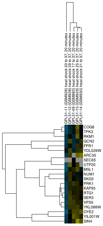
Figure 36. Example export of a portion of a TreeView heat map showing both the Node and Attribute dendrograms (click on the image to see a larger version).
Generally, vector formats yield a higher-quality appearance, as they can be scaled. Particularly for use in a graphics package such as Adobe Illustrator or Adobe Photoshop, vector formats are much preferred. For inclusion in a web page or presentation, png is a reasonable choice if you are not planning on doing any significant zooming and cropping (see Figure 36).
Options for what is included in the output depend on the type of display. For TreeView heat maps that are symmetric (i.e., created using an edge attribute), the Left Node Tree and the Top Node Tree may be included in the output, and you will almost always want to include the Heat Map itself. For TreeView heat maps with both nodes and attributes clustered, you will be able to include the Node Tree, Attribute Tree, and the Heat Map. If the attributes were not clustered, the Attribute Tree will not be available.
If only part of the heat map is desired, you can choose to save just the selected portion (Selection Only). Note that to include dendrograms in the output, you will need to select a full subtree.
- Flip Tree Nodes
- The Flip Tree Nodes button will flip the order of the trees in the top dendrogram, if it exists. At this time, there is no corresponding way to flip the left dendrogram.
- Map Colors Onto Network...
-
The Map Colors Onto Network... button provides a method for mapping the
colors from the heat map back onto Cytoscape nodes (and edges for symmetric heat maps). If a
single column (attribute) is selected, a new VizMap will be created and the colors corresponding to that
attribute will be assigned to the nodes in the network view. If multiple columns are selected, the
Map Colors to Network
dialog (shown in Figure 37 below) will be displayed. From this dialog, you will be able to
select a single attribute and create the VizMap for that attribute, or select multiple attributes to
create a VizMap for each attribute and animate through them. An Animation Speed
slider allows the user to select the speed of the animation. The initial pass will take slightly
longer as the VizMap for each attribute needs to be created, but after that, the animation speed
should correspond closely to the slider. If the nodeCharts plugin is loaded, you will also
be able to create "HeatStrips", which are small bar-charts that represent the heat map values, that
will appear under the corresponding nodes in the network view.
NOTE: At this time, there is no way to save the animation as a movie, although this is a much-requested feature and will be implemented in the future.
- Close
- The Close button closes the dialog.
- Collins SR, Kemmeren P, Zhao XC, Greenblatt JF, Spencer F, Holstege FC, Weissman JS, Krogan NJ.: Toward a comprehensive atlas of the physical interactome of Saccharomyces cerevisiae. Mol Cell Proteomics. 6(3):439–450 (2007). [PMID:17200106]
- Collins SR, Miller KM, Maas NL, Roguev A, et al.: Functional dissection of protein complexes involved in yeast chromosome biology using a genetic interaction map. Nature. 446(7137):806–810. (2007). [PMID:17314980]
- Gasch AP, Spellman PT, Kao CM, Carmel-Harel O, Eisen MB, Storz G, Botstein D, Brown PO.: Genomic expression programs in the response of yeast cells to environmental changes. Mol Biol Cell, 11(12):4241-57 (2000). [PMID:11102521]
- M. B. Eisen, P. T. Spellman, P. O. Brown, and David Botstein: Cluster analysis and display of genome-wide expression patterns. PNAS, 95(25):14863-8 (1998) [PMID:9843981]
- A. J. Saldanha: Java Treeview--extensible visualization of microarray data. Bioinformatics, 20(17):3246-8 (2004). [PMID:15180930]
- M. J. L. de Hoon, S. Imoto, J. Nolan, and S. Miyano: Open Source Clustering Software. Bioinformatics, 20 (9):1453-1454 (2004). [PMID:14871861]
- A.M. Newman, J.B. Cooper: AutoSOME: a clustering method for identifying gene expression modules without prior knowledge of cluster number. BMC Bioinformatics 11:117 (2010). [PMID:20202218]
- L. Apeltsin, J.H. Morris, P.C. Babbitt, T.E. Ferrin: Improving the quality of protein similarity network clustering algorithms using the network edge weight distribution. Bioinformatics 27(3):326-333 (2011). [PMID:21118823]
- B.J. Frey, D. Dueck: Clustering by passing messages between data points. Science 315(5814):972-976 (2007). [PMID:17218491]
- M.E. Newman, M. Girvan: Finding and evaluating community structure in networks. Phys Rev E Stat Nonlin Soft Matter Phys 69(2 Pt 2):026113 (2004).
- G. Su, A. Kuchinsky, J.H. Morris, D.J. States, F. Meng: GLay: community structure analysis of biological networks. Bioinformatics 26(24):3135-3137 (2010). [PMID:21123224]
- A. J. Enright, S. Van Dongen, C. A. Ouzounis: An efficient algorithm for large-scale detection of protein families. Nucleic Acids Research, 30(7):1575-1584 (2002). [PMID:11917018]
- S. van Dongen: Graph clustering by flow simulation [PhD dissertation]. Utrecht (The Netherlands): University of Utrecht. 169 p. (2000)
- T. Nepusz, R. Sasidharan, A. Paccanaro: SCPS: a fast implementation of a spectral method for detecting protein families on a genome-wide scale. >BMC Bioinformatics 11:120 (2010). [PMID:20214776]
- G.D. Bader, C.W. Hogue: An automated method for finding molecular complexes in large protein interaction networks. BMC Bioinformatics 4:2 (2003). [PMID:12525261]
- T. Wittkop, D. Emig, S. Lange, S. Rahmann, M. Albrecht, J.H. Morris, S. Böcker, J. Stoye, J. Baumbach: Partitioning biological data with transitivity clustering. Nat Methods 7(6):419-420. (2010) [PMID:20508635]
- T. Wittkop, D. Emig, A. Truss, M. Albrecht, S. Böcker, J. Baumbach: Comprehensive cluster analysis with Transitivity clustering. Nat Protocol 6(3):285-295. (2011) [PMID:21372810]
- V. Traag, L. Waltman, N. J. van Eck: From Louvain to Leiden: guaranteeing well-connected communities. Scientific Reports 9 (2018) [PMID:30914743]
- M. Rosvall, D. Axelsson, C. T. Bergstrom: The map equation. The European Physical Journal Special Topics, 178(1), 13-23. (2009)
- J. Ramsey, M. Glymour, R. Sanchez-Romero, C. Glymour: A million variables and more: the Fast Greedy Equivalence Search algorithm for learning high-dimensional graphical causal models, with an application to functional magnetic resonance images. Int J Data Sci Anal 3(2): 121-129 (2017) [PMID:28393106]
- I. Inuwa-Dutse, M. Liptrott, I. Korkontzelos: A multilevel clustering technique for community detection. Neurocomputing
- G. Yang, W. Zheng, C. Che, W. Wang: Graph-based label propagation algorithm for community detection. International Journal of Machine Learning and Cybernetics 11(6): 1319-1329 (2020)
- L. McInnesm, J. Healy, J. Melville: UMAP: Uniform Manifold Approximation and Projection for Dimension Reduction. (2020)
- S. Roweis, L. Saul: Nonlinear dimensionality reduction by locally linear embedding. Science 290:2323 (2000)
- M. Belkin, P. Niyogi: Laplacian Eigenmaps for Dimensionality Reduction and Data Representation, Neural Computation 15(6):1373-1396 (2003)
- A.C. Belkina, C.O. Ciccolella, R. Anno, R. Halpert, J. Spidlen, J.E. Snyder-Cappione: Automated optimized parameters for T-distributed stochastic neighbor embedding improve visualization and analysis of large datasets. Nature Communications 10, 5415 (2019).
- I. Borg, P.Groenen:Modern Multidimensional Scaling - Theory and Applications. Springer Series in Statistics (1997)
Result Options
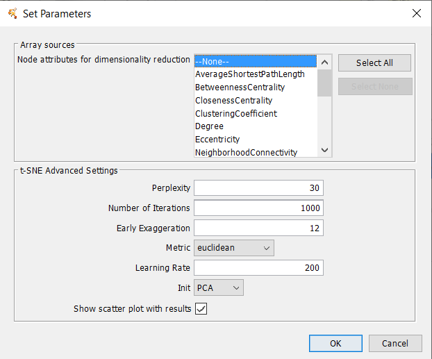
Figure 30. The t-SNE settings dialog.
7.4 t-Distributed Stochastic Neighbor Embedding (remote)
t-SNE is a tool to visualize high-dimensional data. It converts similarities between data points to joint probabilities and tries to minimize the Kullback-Leibler divergence between the joint probabilities of the low-dimensional embedding and the high-dimensional data. t-SNE has a cost function that is not convex, i.e. with different initializations we can get different results. It is highly recommended to use another dimensionality reduction method (e.g. PCA for dense data or TruncatedSVD for sparse data) to reduce the number of dimensions to a reasonable amount (e.g. 50) if the number of features is very high. This will suppress some noise and speed up the computation of pairwise distances between samples.Array Sources
t-SNE (remote) Parameters
Result Options
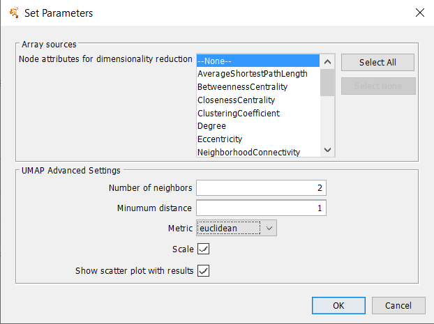
Figure 31. The UMAP settings dialog.
7.5 Uniform Manifold Approximation and Projection (remote)
Uniform Manifold Approximation and Projection (UMAP) is a dimension reduction technique that can be used for visualisation similarly to t-SNE, but also for general non-linear dimension reduction.Array Sources
UMAP Parameters
Result Options
7.6 Isometric Mapping (remote)
Non-linear dimensionality reduction through Isometric Mapping. One of the earliest approaches to manifold learning is the Isomap algorithm, short for Isometric Mapping. Isomap can be viewed as an extension of Multi-dimensional Scaling (MDS) or Kernel PCA. Isomap seeks a lower-dimensional embedding which maintains geodesic distances between all points.Array Sources
Isomap Parameters
Result Options
7.7 Locally Linear Embedding (remote)
Locally linear embedding (LLE) seeks a lower-dimensional projection of the data which preserves distances within local neighborhoods. It can be thought of as a series of local Principal Component Analyses which are globally compared to find the best non-linear embedding.Array Sources
LLE Parameters
Result Options
7.8 Multidimensional Scaling (remote)
Multidimensional scaling (MDS) seeks a low-dimensional representation of the data in which the distances respect well the distances in the original high-dimensional space. In general, MDS is a technique used for analyzing similarity or dissimilarity data. It attempts to model similarity or dissimilarity data as distances in a geometric spaces. The data can be ratings of similarity between objects, interaction frequencies of molecules, or trade indices between countries. There exists two types of MDS algorithm: metric and non metric. In Metric MDS, the input similarity matrix arises from a metric (and thus respects the triangular inequality), the distances between output two points are then set to be as close as possible to the similarity or dissimilarity data. In the non-metric version, the algorithms will try to preserve the order of the distances, and hence seek for a monotonic relationship between the distances in the embedded space and the similarities/dissimilarities.Array Sources
MDS Parameters
Result Options
7.9 Spectral Embedding (remote)
Spectral Embedding is an approach to calculating a non-linear embedding. It finds a low dimensional representation of the data using a spectral decomposition of the graph Laplacian. The graph generated can be considered as a discrete approximation of the low dimensional manifold in the high dimensional space. Minimization of a cost function based on the graph ensures that points close to each other on the manifold are mapped close to each other in the low dimensional space, preserving local distances.Array Sources
Spectral Parameters
Result Options
8. Visualizing Results
clusterMaker2 provides two basic approaches for visualizations: Heat Maps and Networks. clusterMaker2 provides three options for network display: Create New Network from Attribute, Create New Network from Clusters, and three types of heat map display: HeatMapView (unclustered), JTree KnnView. JTree TreeView, and
Figure 32. The network created by clusterMaker2's MCL clustering algorithm for MS/TAP protein-protein interaction data from yeast. The network was created by using Create New Network from Attribute and selecting the option to add inter-cluster edges back.
6.1 Create New Network from Attribute
This menu item can be used to create a network from any numerical attribute, where only the nodes with the same values of the attribute are connected. Note that there is no binning of these values, so using continues values would result in clusters that make little sense. There are two options on the dialog:
6.2 Create New Network from Clusters
This menu item will be selectable if a network cluster algorithm has completed and stored the cluster numbers in a node attribute. When selected, this menu will create a new network that contains only the intra-cluster edges, then layout that network using the unweighted force-directed layout algorithm. All inter-cluster edges will be dropped. If there is value in visualizing the network with the inter-cluster edges also, see the Create New Network from Attribute menu item above. The user interfaces for the heat map displays are very similar. The most complicated is the JTree TreeView, which will be discussed in detail first. The JTree KnnView and HeatMapView (unclustered) will then be discussed briefly, with an emphasis on how they differ from the JTree TreeView.
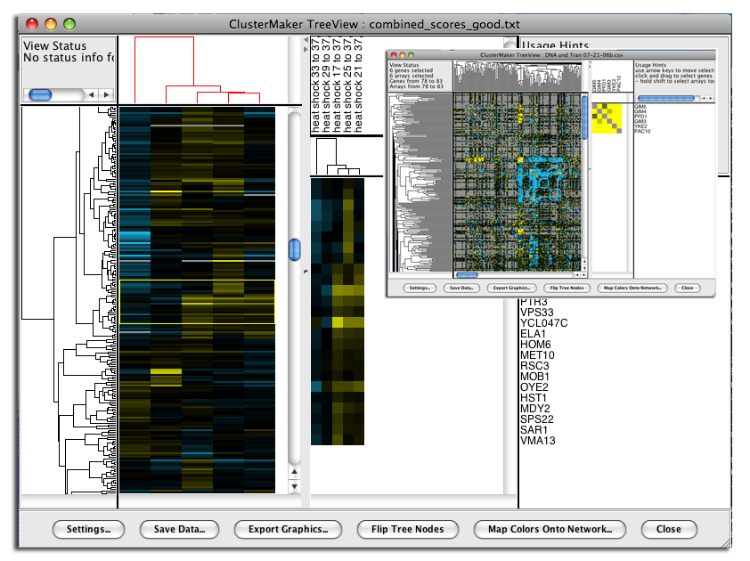
Figure 33. clusterMaker2's JTree TreeView. The larger image shows the results of hierarchically clustering the nodes and five node attributes (expression data from a heat shock experiment). The inset shows the results of hierarchical clustering using an edge attribute. The resulting network is symmetrical across the diagonal, and the dendrograms at the left and top are the same.
6.4 JTree TreeView
Hierarchical clustering results are usually displayed with the JTree TreeView (see Figure 33). This view provides a color-coded "Heat Map" of the data values and the dendrogram from clustering. The JTree TreeView can be created by clicking on the Visualize Clusters button in the Hierarchical cluster dialog (Figure 10) or by selecting Apps→clusterMaker Visualizations→JTree TreeView from the Cytoscape tool bar. Note that both of these methods will be "grayed out" unless hierarchical clustering has been performed on the current network. The information necessary to create the TreeView is retained across sessions (stored in network attributes), so these options should be available when you reload a session that had been saved after hierarchical clustering.The basic TreeView window has four main vertical windows: Node Dendrogram, Global HeatMap, Zoom HeatMap, and the Node List. These windows may be resized to emphasize different portions of the TreeView. Each of the windows is discussed in detail below. Note that selection of a row in TreeView will select the corresponding node in the current network view in Cytoscape (if that node exists). The reverse is also true -- selection in Cytoscape will select the corresponding nodes in TreeView. This is an important feature of clusterMaker2: multiple views (current network, multiple heat maps if present) respond simultaneously to a selection in any one view.
Figure 34. Pixel Settings Dialog.
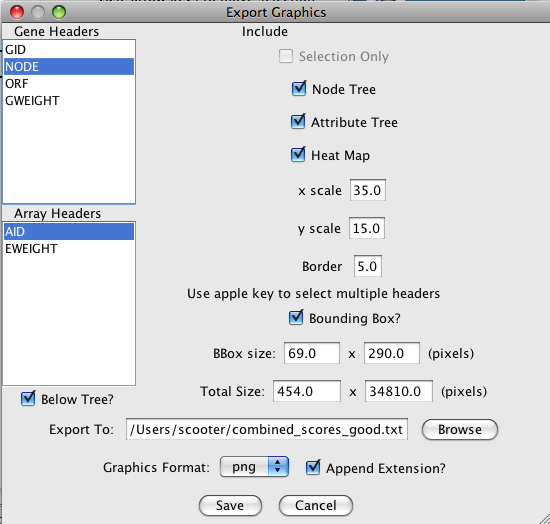
Figure 35. Export Graphics Dialog.
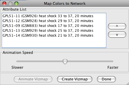
Figure 37. The Map Colors to Network Dialog
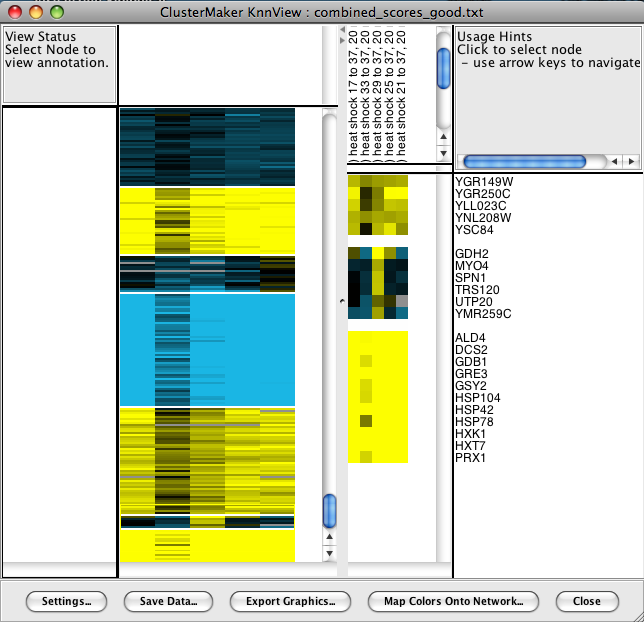
Figure 38. The JTree KnnView dialog showing the results of visualizing a k-Means cluster with k=30.
6.5 JTree KnnView
The results of k-Means clustering can be shown with the JTree KnnView (Figure 38). This is much the same as the JTree TreeView discussed above, except that the dendrogram areas are empty and the clusters are separated by a blank space the width of one cell. All of the features discussed as part of the JTree TreeView are available in the JTree KnnView except the Flip Tree Nodes button, and the Node Tree and Attribute Tree options are not available in the Export Graphics dialog.6.6 HeatMapView (unclustered)
Any attribute or group of attributes may be shown as a heat map using the clusterMaker2 HeatMapView (unclustered). The dialog is identical to the JTree KnnView except that since there are no clusters, there are no blank spaces separating the clusters.7. Interaction
7.1 Link network selection
This capability is planned, but not yet implemented in clusterMaker2
8. Acknowledgements
The Hierarchical and k-Means implementations of clusterMaker2 are based on the Cluster 3.0 C implementation (from Michiel de Hoon while at the Laboratory of DNA Information Analysis at the University of Tokyo), which was based on the original Cluster program written by Michael Eisen. The heatmap/dendrogram visualization is based on Java TreeView implemented by Alok Saldanha while at Stanford University. The MCL cluster algorithm was written based on the original thesis by Stejn van Dongen, with reference to the Java implementation by Gregor Heinrichi (see http://www.arbylon.net/projects/knowceans-mcl/doc/).
9. References
About RBVI | Projects | People | Publications | Resources | Visit Us
Copyright 2018 Regents of the University of California. All rights reserved.